We discussed logistic regression in a previous article.In this article we will explore how to do logistic regression the bayesian way using the rstanarm package in R.
The benefit of taking a bayesian approach is that it allows us to model the uncertainty in our parameter estimates directly.
Below we explore Bayesian logistic regression for explaining customer choices between two products, and run a simple scenario to determine how changing the price is likely to impact the probability of selection.
Simulating Data
We will use the same simulated data set as we did in part one, where 1 indicates a customer chose a smoothie and 0 indicates they chose a milkshake.
library(tidyverse)
library(statmod)
library(rstanarm)
options(mc.cores = 4)

InvLogit <- function(x) {
  exp(x)/(1+exp(x))
}

set.seed(123)
Sex <- rbinom(1000, 1, 0.25)
Price <- rnorm(1000, 10, 3)
# Sunday to Saturday
Day <- sample(1:7, 1000, T) - 1
Income <- sample(seq(50, 150, by = 10), 1000, replace = T)
Raw <- InvLogit(((Day * .2) + (Price * -0.2) + (Sex * .02) + (Income * .02) + rnorm(1000, 0, 0.1)))

Data <- data.frame(cbind(Sex = Sex, Price = Price, Day = Day, Income = Income, Prob = Raw))
Data$Choice <- rbinom(1:1000, 1, Data$Prob)
Bayesian Model
Rstanarm makes it very simple to run a bayesian binomial model. The only difference, assuming we are fine non-informative priors, is the function is stan_glm().
glm.stan <- stan_glm(Choice ~ Price + Day + Income,
family = "binomial", data = Data)

summary(glm.stan, probs = seq(0,1, by = .1))
We can also add a weakly informative prior to our model. This will increment the log probability mass function in Stan with the value of the prior which operates to constrain the estimate and can help with model fit.
We can set a weak normal prior on our predictors with the prior parameter. This would be more important if we had a smaller dataset, with 1,000 observations the prior will get washed out very quickly.
glm.stan <- stan_glm(
  Choice ~ Price + Day + Income,
  family = "binomial",
  data = Data,
  prior = normal(0, 1)
)

summary(glm.stan, probs = seq(0,1, by = .2))
In this case, the estimate of Day ends up being a little more stable after being constrained by the prior. In the previous article there were some issues with our right tail not being exactly normal, so this is a welcome development.
There are many priors available in rstanarm and they can be set on the predictors, covariance, or the intercept as required.
Diagnostics
We also want to check our Rhat values to ensure they are all at 1.0 as that indicates that the four chains have converged. Lack of convergence indicates problems in the model which will cause problems with estimation.
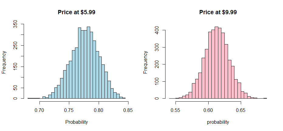
We can plot out histograms to give ourselves an understanding of the expected value and credible range of probability outcomes, given the two smoothie pricing scenarios.
par(mfrow = c(1,2))
hist(Distro$Choice, breaks = 50, col="lightblue",
xlab = "Probability", main = "Price at $5.99")
hist(Distro2$Choice, breaks = 50, col="pink",
xlab = "probability", main = "Price at $9.99")
Unsurprisingly, the probability of purchasing a smoothie is higher with a lower price. However, the benefit of this approach is that we can understand the range which can be helpful for sensitivity analysis.
The bayesian approach also shows us that these distributions do not overlap, the difference is large enough that we are unlikely to see the same results at $9.99 as we would at $5.99. In other words, the worse case $5.99 scenario is expected to exceed what $9.99 is capable of.
Differences
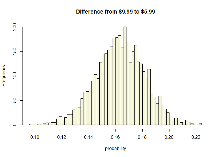
Since we have simulated outcomes to work with, we can also easily visualize the expected difference in range by simply subtracting one vector from the other.
Diff <- Distro - Distro2
par(mfrow = c(1,1))
hist(Diff$Choice, breaks = 50, col="beige", xlab = "probability",
     main = "Difference from $9.99 to $5.99")
We can see that the expected difference is 0.16 over a range of 0.10 to 0.22 on the probability scale. This is much easier to work with and communicate than traditional methods.
The difference in means, and variance will be the same as in manual calculations. Note that VAR(X)-VAR(Y) is equal to the the covariance of differences.
The bayesian method is simpler and easier to work with than prediction confidence intervals. More importantly, it is easier to communicate.
Conclusion
Stan, the rstanarm package, and advances in computing power have made Bayesian data modeling incredibly convenient. This is a great approach for business intelligence where we may want to incorporate prior knowledge, and understand the bounds of risk and reward.
There are huge benefits to getting familiar with this approach, and rstanarm is a great way to start.
References
Matsurra, K. Bayesian Statistical Modeling with Stan, R, and Python. Springer, 2022.
Gelman, A; Carlin, J. et al. Bayesian Data Analysis, 3rd Ed. Chapman & Hall/CRC, 2013.