Transformations are changes to our response variable that can be employed to solve issues such as a lack of homogeneous variance, or to make interpretation easier as in the case of the log-log price elasticity model.
MLR3 Pipelines provides an automated way to handle transformations and where required also to transform back to the original scale during prediction.
Let’s explore a few ways to use transformations with the MLR3 package and mlr3pipelines in particular.
Dataset
We will use a freely available Kaggle dataset that lists car prices based on an assortment of features such as length, horsepower, and city mileage.
Preparing Data
First we will do some preparation on our dataset and create a regression task.
For this example we will create a single regression learning using glmnet.
GLearner = lrn("regr.glmnet",
               id = "GlmModel",
               s = to_tune(p_int(0, 15)),
               alpha = to_tune(p_dbl(0, 1))
)
Independent Variables
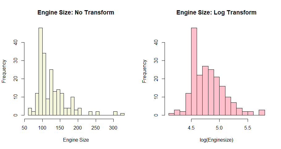
The engine size variable is not normally distributed, for a demonstration of the mutate functionality we will apply a log transformation. In this case it seems to help somewhat but there there is still a lot of density near 4.5 on the log scale.
Note that there are specific pipeline operators for common transformations such as Box-Cox or Yeo-Johnson, using these operators may be preferable where we don’t need the flexibility of a customized mutation function.
par(mfrow=c(1,2))
hist(CarMod$enginesize, breaks = 20, main = "Engine Size: No Transform",
xlab = "Engine Size", col="beige")
hist(log(CarMod$enginesize), breaks = 20, main = "Engine Size: Log Transform",
xlab = "log(Enginesize)", col = "pink")
Transformation Pipeline
We’ll create a piece of pipeline that performs feature encoding of categorical features, then a log transformation on engine size, and finally a log transformation on the target.
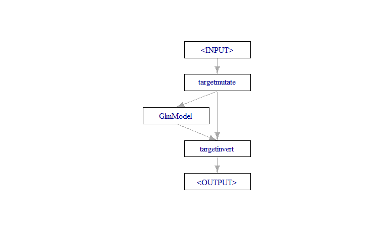
The final step uses a pre-built pipeline availabe in in mlr3 called pipeline_targettrafo which sets up the target transformation. The TRAFO module contains a mutation step that passes the transformed target to a learner along with an inversion function. From there the inverter will call that function to carry out the back transformation.
This can be created from scratch with the target mutate and target invert pipe operators but using the existing pipeline for a standard procedure saves time and avoids having to worry about which inputs are going into which output channels of the component operators.
The learner we are specifying below is simply a clone of the above glmnet model, including the same tuning tokens.
Note that while the manual suggests specifying the inverter function as a named list we found simply using exp(x) in the inverter function call correctly mapped it to the response variable as it does in the trafo function.
Next we will build out the remainder of the transformation pipeline by first converting this section into an integrated learner with as_learner() and then using the pipeline graph constructor %>>% before plotting the result.
Once our mutations are set up we can tune our hyperparameters as usual. A more detailed explanation is available in another article Benchmarking Vehicle Prices with MLR3. However, essentially we are specifying a tuning strategy, in this case Bayesian optimization for 120 seconds using 3 fold cross validation.
The entire pipeline we created will be tuned over as a unified learner when hyper parameters are selected. In addition when we have new data for predictions the transformations will also be applied to the new data.
Our RMSE is 1,953 and our predictions have been back transformed as intended.
Conclusion
MLR3 is a flexible machine learning package, and it also provides plenty of flexibility to use transformations on both the target and feature variables. Before setting up your own target transformations be sure to check whether there are pre-built pipe operators such as PCA, scale, Box-Cox, and Yeo-Johnson.