We often have to consider a lot of variables in exploratory analysis, but like most problems breaking our data down into components can speed up finding solutions. With business data we often don’t have the luxury of spending hours with experts or days pouring over customer attributes.
Principal Component Analysis is a good friend to have for exploratory work. We can use PCA to get a sense of how our numeric variables are correlated and also which ones provide unique information.
Let’s explore how we can use PCA to get a sense of which factors have an impact on car prices.
Dateset
We will use a freely available Kaggle datasetthat lists car prices based on an assortment of features such as length, horsepower, and city mileage.
Results
We narrow down variables that impact price into four components and identify key relationships between price and other variables. Specifically, there is a tradeoff between fuel economy and engine strength along with car size, but price follows engine size.
Follow along below in R studio to see how we arrived at this result.
Data Loading
First we will load our dataset and remove some of the less relevant variables, and also the non-numeric variables. PCA only works for numeric variables. For cylinder count we will transform it to an integer.
We will also load the packages factoextra and FactoMinR, these packages make working with PCA a breeze.
Principal Component Analysis (PCA) is intended to reduce the number of explanatory variables without losing information. To do that it compresses the features into a number of information dense components that are made up of combinations (mixed proportions) of the originals.
The first step in our analysis is to run PCA on the numeric dataset. We will leave Price included even though it is our dependent variable just to see which other variables it moves with.
Note that the PCA function defaults to centering and scaling our variables and keeping five components which are sensible defaults.
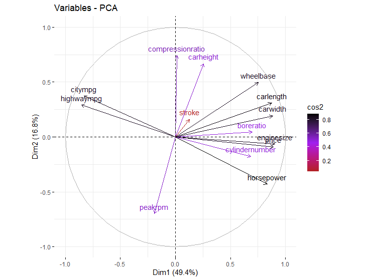
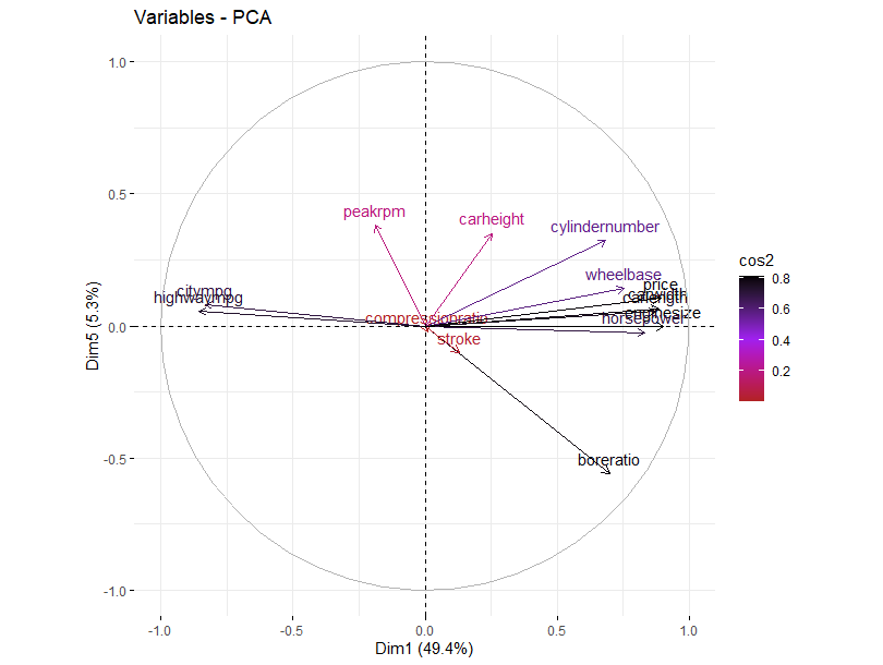
Next, the function fviz_pca_var() allows us to visualize the contribution on a circle of correlations. Lines that move in the same direction are positively correlated and those in the opposite direction are negatively correlated.
For this data price tends to move in the direction of engine size, horsepower, and cylinder number. Those features move, unsurprisingly, in the opposite direction of both city and highway mpg.
The length of the lines represents how well they are represented across the two components that have been graphed called Dim1 and Dim2. These are first two information dense components produced by PCA. Most of our variables are well represented, but stroke is not, suggesting that it contains different information that may not be relevant considering that it is uncorrelated with price.
Revisiting PCA
Although including price is helpful to give a glimpse of what might be relevant for analysis, we should keep the dependent variable out of PCA components or it will cause problems with modeling. We want to understand how our components correlate with price, and this will not be possible if we include part of the price information in a component.
As we can see, with price removed the components are essentially the same, except that they no longer have any information residue from price in them.
Roughly speaking, we have three relevant groups of variables. One has to do with mileage, another with engine strength, and a third with vehicle size. The later two move imperfectly together in the same direction, and mileage moves in the opposite direction.
There is a trade off between engine size and care size on one hand, and mileage on the other; and we know that price follows engine.
Exploring Components
To explore the components we can extract the eigen values. These relate to matrix algebra where a transformation is applied to a vector, and this stubborn vector ends up not changing direction, only its scale becomes larger or smaller. In that case, the eigen value is the amount of scaling that resulted from the transformation.
For exploratory analysis these values are not really important except that they relate to the proportion of variance explained by each principal component. This is conveniently calculated in the second and third columns below.
eigen <- get_eigenvalue(comp)
eigen
fviz_eig(comp, addlabels = T)
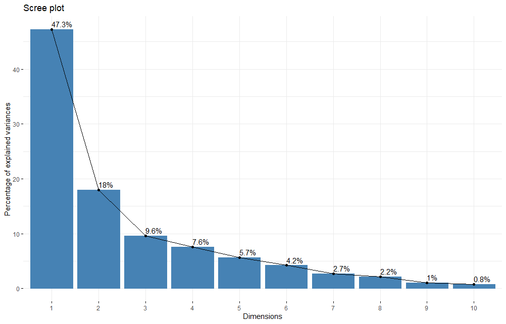
This cumulative variance can be represented in a scree plot which helps us make decisions on how many components to include in our analysis.
fviz_eig(comp, addlabels = T)
Looking at the scree plot suggests two very relevant components followed by some less relevant but not insignificant components. The first three components capture over 70% of the variance in our feature set, and with the fourth it is over 80%.
After some point we get diminishing returns, so we would want to select a number of components based on the amount of variation we would like to retain and the amount of features we want to keep, bearing in mind that the goal is to reduce the number of features to the extent possible.
Looking around the “elbow” of the plot gives a good starting point. We might keep 3 or 4 components which is very close to 95%. If we can get away with three that might be a better choice because it will be easier to explain.
Plotting Components
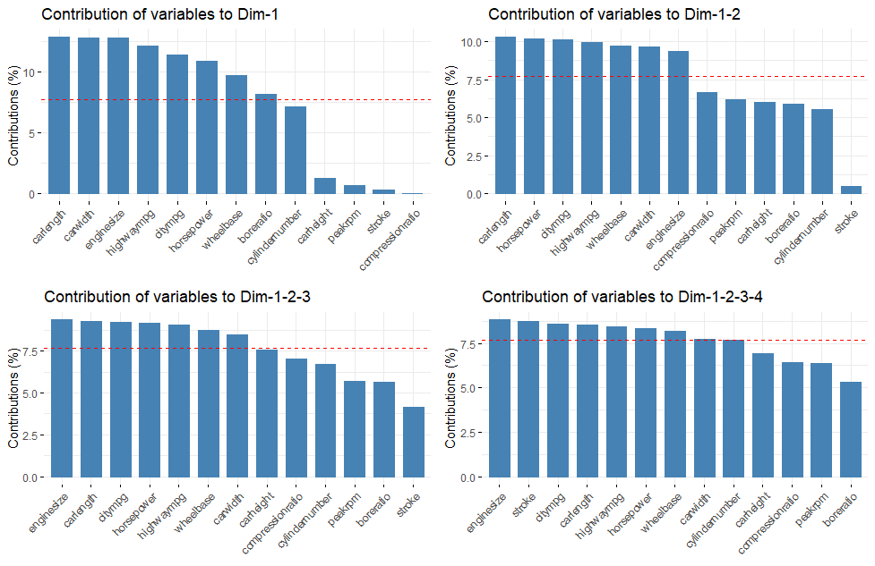
Plotting out the components is a helpful way to decide if we have everything we need included. We can use the gridextra package to make multiple ggplots. The axes parameter in fviz_contrib() is used to specify a vector of components. Chart one shows component 1, and chart 4 show the cumulative of components 1 through 4.
The red line in these plots indicates the expected contribution of components if they all made the same contribution. That means variables above the line are contributing more than expected to the component, or group of components.
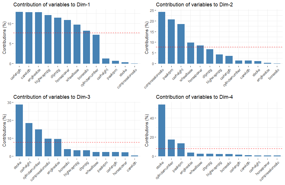
We can also look at each component indivually to see what pops out.
If we keep four components we will get a bit more of cylinder number and a fair bit of stroke. Both of these components were correlated with price so including them might help predictions.
Corr Plots
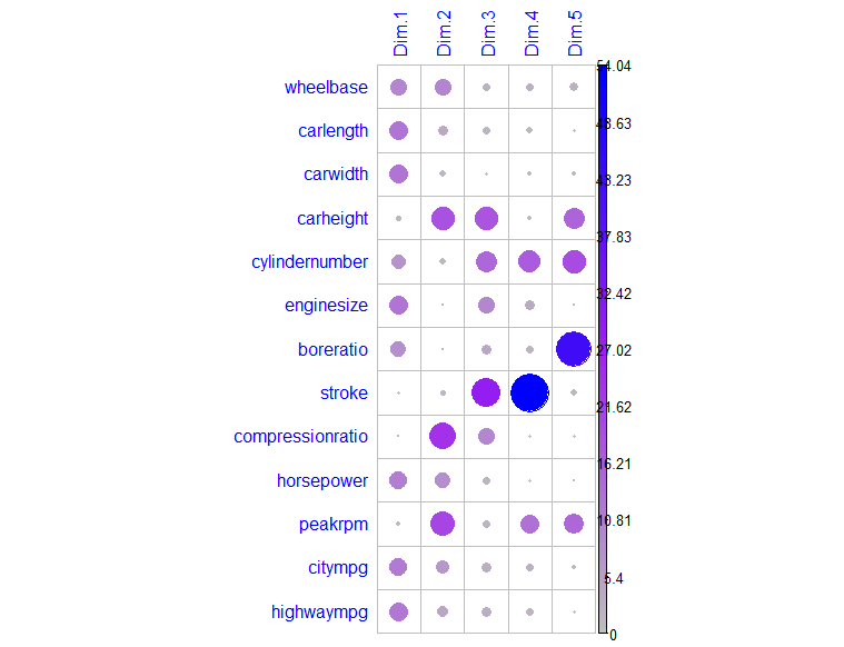
We can also use the corrplot package to vizualize the contribution of our variables to the components.
This layout makes it easier to view more components. Notably, if we are interested in bore ratio then we may want to keep component five. If we are interested in stroke then we will want to keep component 4. Cylinder number is spread across Dim3 to Dim5.
Selecting Components
Depending on our goal we might decide to keep 3-5 components, and we could test models with different numbers of components to see what gives the best result.
Although it is tempting to keep components up to some number because they are named 1-5, there is no rule saying we must keep 2 if we keep 3. Obviously, we will want to keep the components that explain a lot of variation but we can also consider our objective.
Unless we want five components, there is a 2% difference between 4 and 5, except that if our goal is to understand price then component 5 contains bore ratio which is correlated with price. Importantly, bore ratio is also different from other variables correlated with price which is why it is in it’s own component.
Component 4 contains stroke which was not correlated, so we will probably get better results by preferring 1 and 5. We will also keep 2 and 3, although they are largely centered on components we do not care about, they are large and they contain information about horsepower and cylinder number.
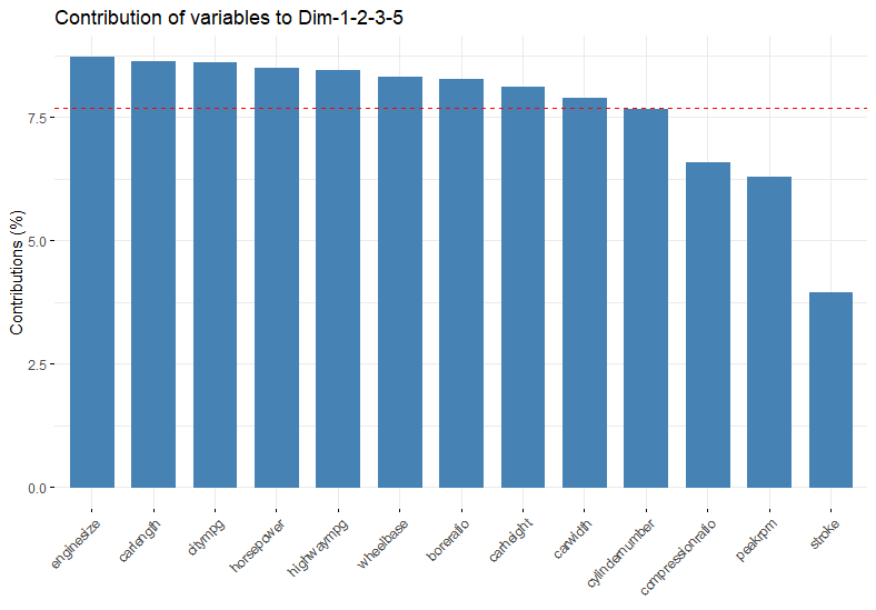
The contribution graph for this choice is shown below, where we have at least average contribution from all of the variables that we care about from our original correlation circle which we can plot again this time with components 1 and 5 on the axes.
We might say component one has to do with economy, including car size, and engine size. Component two has to do with compression and form factor. Component three and five with different aspects of engine performance.
Of course this is all exploratory. Now that we have a better understanding of our data and what to expect in analysis, we will want to run a proper model using price as our target variable.
Conclusion
Although principal component analysis is intended to reduce the number of variables we have to worry about, it is also a helpful way to explore new data quickly with very little coding.
There are automated feature selection tools like stepping through AIC scores but these are poor substitutes for getting to know the data especially as the number of features grows.
If we can represent a large number of attributes numerically, PCA becomes a friend that helps us identify relationships in our data, along with meaningful ways to group things together. That speeds up the exploratory data process and helps us make more informed modeling decisions.