Stacked Regression Pipelines in MLR3

Dustin

25 June 2024
9 min read

Introduction

The mlr3 ecosystem provides a powerful and comprehensive set of packages that attempts to unify machine learning with R. The packages provide a modular approach centered around functional tasks such as learners, tasks, tuning, and pipelines.

This article will explore creating a stacked regression model in mlr3 based on three learners fed into an optimized averaging component that we can use to make predictions on vehicle prices.

Dataset

We will use a freely available Kaggle dataset that lists car prices based on an assortment of features such as length, horsepower, and city mileage.

Loading Data

First we will load required packages and our data, and get rid of a few features that are unnecessary given the dataset scenario of determine important pricing features for a potential new product launch.

We also transform cylindernumber into an integer variable to cut down the number of parameters required in our model.

library(tidyverse)
library(mlr3verse)
library(mlr3filters)
library(mlr3extralearners)

CarPrices <- read.csv("CarSales.csv", stringsAsFactors = T)

CarPrices$curbweight <- NULL
CarPrices$symboling <- NULL
CarPrices$CarName <- NULL
CarPrices$car_ID <- NULL

CarMod <- mutate(CarPrices,
                 cylindernumber = case_when(
                   cylindernumber == "one" ~ 1,
                   cylindernumber == "two" ~ 2,
                   cylindernumber ==  "three" ~ 3,
                   cylindernumber == "four" ~ 4,
                   cylindernumber == "five" ~ 5,
                   cylindernumber == "six" ~ 6,
                   cylindernumber == "seven" ~ 7,
                   cylindernumber == "eight" ~ 8,
                   cylindernumber == "twelve" ~ 12
                 )
)

Task Module

Our first task is to define a task. We will set up a new regression task using our modified car data (CarMod) as the backend dataframe.

## Task Definition
PriceTask <- TaskRegr$new(
  id = "PriceTask",
  backend = CarMod,
  target = "price"
)
PriceTask$col_info

Learner Modules

The next stage of creating a stacked learner is to create a few learners and set up their tuning parameters. The learner mechanics are beyond the scope of this article but we will set up three of them as part of the demonstration of pipelines.

Penalized regression (glmnet)
Random Forest
MARS (multivariate adaptive regression splines)

Conventional wisdom is to use different types of learners in order to maximize the benefit from stacking because each has strengths and weaknesses. The idea is that strengths in one model will compensate for weaknesses in another.

### Learners
GLearner = lrn("regr.glmnet",
  id = "GlmModel",
  s = to_tune(p_int(0, 15)),
  alpha = to_tune(p_dbl(0, 1))
  )

RFLearner = lrn("regr.randomForest", 
                id = "RFModel",
                ntree = 300,
                mtry = to_tune(p_int(5,12)),
                nodesize = to_tune(p_int(1,5)),
                maxnodes = to_tune(p_int(5,20))
)

MLearner = lrn("regr.mars", 
                id = "MarsModel",
                degree = to_tune(p_int(1,3)),
                nk = to_tune(p_int(1,200))
)

Pipe Operators

Below we will set up three pipe operators with the po() function. This is what mlr3 calls a “sugar” function which is a convenient setup function that is short and avoids having to deal with the somewhat irritating R6 class behaviour.

MLR2 functions were notoriously long winded so having sugar functions makes development a much more pleasant experience.

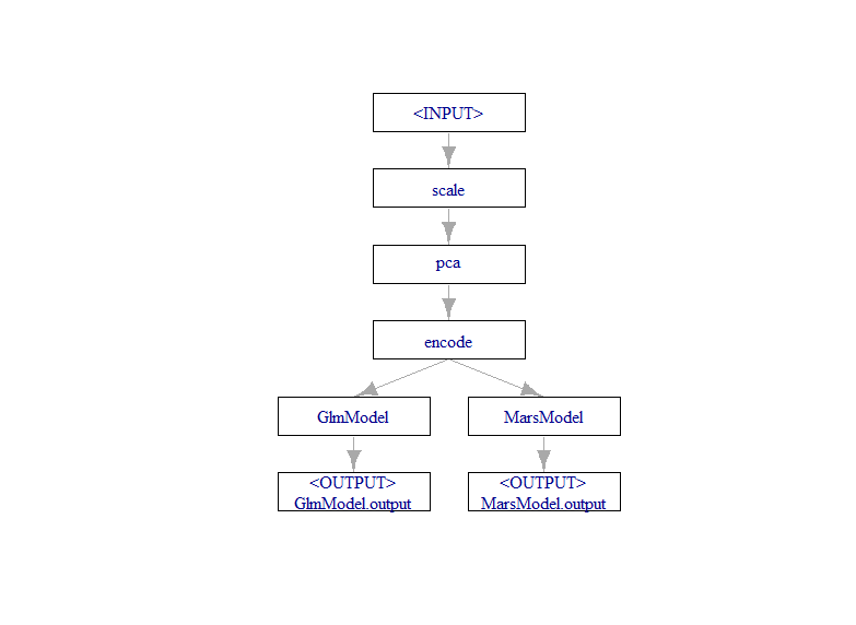
The first component is a feature encoder that will transform our factor variables into a one-hot-encoded form. The second is a scale operator that will scale and center our numeric variables. The third is a Principle Component Analysis operator that will perform PCA on the scaled input.

For PCA we specify center as false, this is because it will be fed by scale operator. We will also tune the number of components to keep from 3 to 6 with the “rank.” parameter. Note that some parameters end with a “.” which is a bit confusing, and PCA defaults to centering without scale.

Encoder <- po("encode")
Scaler <- po("scale", robust = T)
PCA <- po("pca", center = F, rank. = to_tune(p_int(3,6)))

There is a massive and growing list of operators and templates available in the documentation. We can also design our own by inheriting from the base pipeline operator classes using the R6 framework.

Graph Union

The next component of our pipeline is a graph union object which is passed a list of learners, in this case the two learners we plan on attaching to our preprocessing steps above.

PartTrain <- gunion(
  list(
    GLearner,
    MLearner
  )
)

Building Pipelines

In order to attach components together we need to use the %>>% operator. This is a short hand function for creating graphs that replaces a rather obnoxious chain of R6 class bindings that would otherwise be necessary to chain components together.

We are creating a graph object called RegPipe and specifying the order of the components. The order is important, first we scale, then apply PCA, and follow with the encoder. Putting the encoder first would result in our dummy variables being scaled and turned into components which is not what we want.

RegPipe <- Scaler %>>% PCA %>>% Encoder %>>% PartTrain 
plot(RegPipe)

This completes our first section of pipeline that includes preprocessing and two learner models.

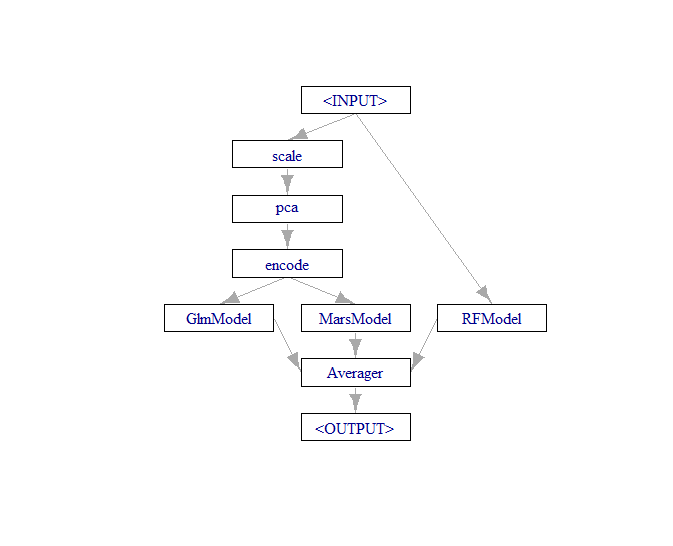
Adding More Learners

This is where the fun begins, now we can perform another graph union, but this time between the pipeline object and our third learner that will be excluded from the preprocessing steps.

We will also feed the new union object (which contains the entire pipeline above plus the new learner) into an optimized averaging component that will attempt to learn the best weighted average of our three predictions.

FullTrain <- gunion(
  list(
    RegPipe,
    RFLearner
  )
)
FinalTrain <- FullTrain %>>% po("regravg", id = "Averager")
plot(FinalTrain)

Pipeline Learner

The final step before we can get into training is to convert our pipeline into a learner.

This is one of the features that makes mlr3 such a great package. The entire complex pipeline will now operate as a cohesive unit in tuning, training, and prediction.

This means that during cross validation all of the learners will get the same split of data to work on, our preprocessing steps will be tuned, and making predictions afterward with new data will be quick and easy.

FinalLearner <- as_learner(FinalTrain)

Tuning the Pipeline

Without getting too caught up in the details. We are splitting our data into a training and test set and then deciding on a tuning strategy.

We will use 200 seconds of training using a Bayesian optimizer. As with all things mlr3 it is possible to customize the tuning approach, termination approach, and even customize the Bayesian optimization approach if you are so inclined.

We will use a multi-session parallelization plan with five worker processors. Our resampling strategy will be five fold cross validation.

The instance is our tuning instance, once this code is run mlr3 will begin to tune our pipeline learner and provide parameter results that we can use to train our model.

### Split Data
Splits = partition(PriceTask, ratio = 0.9, stratify = T)

## Tuning Strategy
terminator = trm("run_time", secs = 200)
tuner = tnr("mbo")
measure = msr("regr.rmse")

future::plan("multisession", workers = 5)

### Tuning

instance = tune(
  tuner = tuner,
  task = PriceTask$filter(rows = Splits$train),
  learner = FinalLearner,
  resampling = rsmp("cv", folds = 5),
  measures = measure,
  terminator = terminator
)

future::plan("sequential")

instance$result_learner_param_vals
instance$result

Model Training

The final step is to create a deep clone of our FinalLearner pipeline object which we will called FinalTuned.

Next we will assign the optimal parameters to our pipeline learner, and train it on our test data by specifying the row_id from our partition.

#Train Final Model

FinalTuned = FinalLearner$clone()
FinalTuned$param_set$values = instance$result_learner_param_vals
FinalTuned$param_set$values

FinalTuned$train(PriceTask, row_ids = Splits$train)$model

Holdout Validation

Now we can see how our stacked learner performed on our validation set using RMSE as the metric.

ResultsEL <- FinalTuned$predict(PriceTask, row_ids = Splits$test)
sqrt(mean((ResultsEL$truth - ResultsEL$response)^2))

> sqrt(mean((ResultsEL$truth - ResultsEL$response)^2))
[1] 1630.942

Our model gets very decent performance for 200 seconds of training time on unseen data.

Benchmarking

Benchmarking in mlr3 is also easy to setup. There is a featureless learner available to use as a baseline which we will use to benchmark against. However, nothing stops us from creating several pipeline options and testing to determine which one has the best performance.

BaseLearner <- lrn("regr.featureless")
Learners <- list(BaseLearner, FinalTuned)
BenchTask <- list(PriceTask)

Experiment <- benchmark_grid(
  tasks = BenchTask,
  learners = Learners,
  resamplings = rsmp("cv", folds = 5),
)
Experiment

BenchResult <- benchmark(Experiment)
BenchResult$aggregate(msr("regr.rmse"))

                                             learner_id regr.rmse
                                                 <char>     <num>
1:                                     regr.featureless  7775.075
2: scale.RFModel.pca.encode.GlmModel.MarsModel.Averager  2499.186

Running 5 fold cross validation, our pipeline performs significant better than the baseline learner.

Normally benchmarking will be more optimistic than real world performance, but our learner had much better performance on the validation set. This might reflect some instability which we can check by looking at the individual folds.

BenchResult$score(msr("regr.rmse"))[,c("learner_id", "regr.rmse")]

                                               learner_id regr.rmse
                                                  <char>     <num>
 6: scale.RFModel.pca.encode.GlmModel.MarsModel.Averager  2141.982
 7: scale.RFModel.pca.encode.GlmModel.MarsModel.Averager  2063.730
 8: scale.RFModel.pca.encode.GlmModel.MarsModel.Averager  2488.982
 9: scale.RFModel.pca.encode.GlmModel.MarsModel.Averager  3137.140
10: scale.RFModel.pca.encode.GlmModel.MarsModel.Averager  2664.098

There is a bit more instability than we would ideally like to see, but it’s a good start for 200 seconds of training on a complex model. Thankfully, mlr3 makes it very easy to go back and adjust a few things like the number of PCA components to tune on, or even swap out a learner.

Conclusion

MLR3 is a great machine learning package for R. It is a bit more of a rabbit hole than tidymodels but the level of flexibility and control it provides make it well worth getting familiar with the various packages and features.

The flexible pipelines available in mlr3pipelines are an extremely useful extension that covers a vast array of standard machine learning operations. Best of all, you can always create your own if you don’t find what you are looking for.

References