Classification involves grouping things together based on shared qualities. This process can be automated to assign newly acquired customers into segments, or to help us understand what products our customers are most likely to be interested in.
Let’s explore how we can build a machine learningpipeline in MLR3 to determine which product to market to a group of customers.
Scenario
We will set up a pipeline to classify customers by the type of sewing machine they are most likely to purchase given the age, gender, skill level, income, and years of experience.
In an effort to keep things relevant the headings have been renamed. “Drug” has also been replaced with “Product” in the target column.
We will rely on MLR3 for our model. This is a machine learning framework for R that consolidates a huge number of algorithms and provides a common interface and pre-processing pipelines.
Results
We create a machine learning model and use it suggest the best product to promote to a new customer, and that is Product Y (pictured above).
Follow along below in R Studio to see how we arrived at this result.
Loading theData
First let’s load a CSV of the modified Kaggle data importing text fields as factor variables. Since R is case sensitive we also ensure target variable is spelled consistently by setting it to all upper case letters.
We will also set options(mc.cores = 4) to specify available 4 processor cores for any parallelization in training. That is using more than one processor to save time.
    Age        Sex        Skills      Income      Experience         Product
 Min.   :15.00   F: 96   HIGH  :77   HIGH  :103   Min.   : 6.269   PRODUCTA:23
 1st Qu.:31.00   M:104   LOW   :64   NORMAL: 97   1st Qu.:10.445   PRODUCTB:16
 Median :45.00           NORMAL:59                Median :13.937   PRODUCTC:16
 Mean   :44.31                                    Mean   :16.084   PRODUCTX:54
 3rd Qu.:58.00                                    3rd Qu.:19.380   PRODUCTY:91
 Max.   :74.00                                    Max.   :38.247
>
Data Balance
These summary statistics show us the range of our continuous variables, and the balance of our categorical variables. Sex, Skills, and Income seem balanced, however our target class (“Product”) is unbalanced.
Class imbalance is likely to result in a poorly trained model. Imagine if our dataset had 90% “Yes” and 10% “No.” If we guess “Yes” every single time then our classification error will be very low even if our model is no good. This is something we will try to correct in our pipeline.
ClassificationTask
The first step with MLR3 is to define a task. Tasks can include regression, clustering, survival, and various others. In this case we are classifying so the obvious choice is a classification task. We specify the target as the “Product” column and examine data again.
Key: <id>
           id    type       levels  label fix_factor_levels
       <char>  <char>       <list> <char>            <lgcl>
1:   ..row_id integer                <NA>             FALSE
2:        Age integer                <NA>             FALSE
3: Experience numeric                <NA>             FALSE
4:     Income  factor HIGH, NORMAL   <NA>             FALSE
5:    Product  factor productA....   <NA>             FALSE
6:        Sew  factor PRODUCTA....   <NA>             FALSE
7:        Sex  factor         F, M   <NA>             FALSE
8:     Skills  factor HIGH, LO....   <NA>             FALSE
>
We will also split our data into training and test, setting aside 10% of 200 observations for validation. We then stratify to ensure that we get a good representation of the difference product classes.
We will use an algorithm called Support Vector Machines (SVM) to classify our customers. These models create divisions in space to separate in and out groups based on their properties. Kind of like drawing a line in the sand.
The challenge we will have using this type of model is that they can’t handle categorical variables in the feature set, only the target can be a factor. This is something we will have to address in our machine learning pipeline.
First we will define our learner and tell it which “Hyper Parameters” we want to tune on. These parameters are the dials that we need to set in order to get the best results from the model.
We will tune on the basic parameters (cost, gamma, degree) that affect model predictions. Tuning is just trying different settings to see what combination of parameters lead to the best results given our data.
It is also possible to tune the type of kernel bearing in mind that not all parameters apply to all kernels which creates dependencies.
Sampling Parameters
Next we will define some parameters to help tune our model. We will use three fold cross validation for testing the accuracy, and a simple grid search as a tuning strategy. We will search the grid trying different parameters with the goal of minimizing classification errors.
Grid searches exhaustively try every combination of parameters according to the resolution. We use a low resolution to avoid hours of anticipation and excess carbon consumption.
The time has come to address the major issues in our dataset. The first is class balance, and the second is that our factors will cause SVM to complain since it needs numbers not categories.
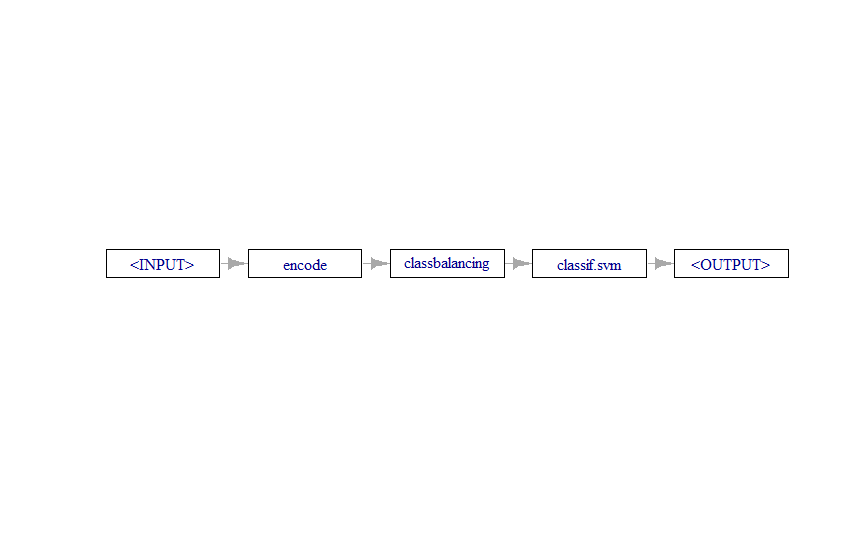
MLR3 provides for the construction of pipe operators which are data pre-processing steps and graphs which are a flowchart of these pre-processing steps that lead to the learner.
We will use a balancer po(“classbalancing”) and set the reference to “major” which tells the balancer to use the largest target class as a reference. We do this because we want to bring the smaller classes up rather than bring the larger class down by throwing away data.
The balancer will randomly up-sample the small classes so that they are the same size as the large classes. This is not always an ideal solution, we might want to set penalization weights instead, or try both and benchmark to see which approach gets better results.
The second step is an Encoder that transforms categorical features defined as Factors in R into numeric data. For example, Sex (“M”, “F”) becomes Sex.M = 0 and Sex.F = 1.
Finally, we combine both of these steps into a graph with our learner using the %>>% operator which tells MLR3 how to join our pipeline steps together into a graph.
The final step is to turn our graph into a learner with as_learner(graph). This is just taking the entire pipeline and letting MLR3 know to treat it as a learner.
In order to get the best idea of how our model will generalize to new data in the real world we will run a layered resampling. Since it is computationally expensive we will assign three worker cores.
Once finished, we will extract the results and see what to expect from our proposed SVM model on this data.
Classification error is estimated to generalize to about 5%, depending on the application this could be good or bad but we will assume it is fine for advertising our sewing machines.
We filter our task to include only the training data from our partition to avoid any unnecessary data leakage taking place. Data leakage can cause the model to be over-fit and have trouble generalizing.
Model Tuning
We get acceptable cross validated test results, and they seem to remain stable across runs. We can now move on to tuning our model on the training data. This will provide the best estimate for our hyper parameter settings.
Model fit looks even better now with a 3.9% classification error, but recall that our best real world estimate is about 5%. We should avoid relying on the training classification error of the tuned model to predict real world performance. This is why we used the layered tuning approach above to benchmark.
Final Training
We will now take the parameters from tuning and put them into a newly created model that will be cloned from our pipeline (“PipeLearn”).
Next we train the model on our training set partitioned earlier.
#Train Final Model
PipeTuned = PipeLearn$clone()
PipeTuned$param_set$values = instance$result_learner_param_vals
PipeTuned$param_set$values

PipeTuned$train(SewTask, row_ids = Splits$train)$model
Now that we have a trained model, let’s see how it performs on our test set. We can use a “confusion matrix” to visualize the number of times the prediction was the same as the ground truth, that is whether our model was correct or not.
Our model has a 95% prediction performance for 20 observations from a test set it hasn’t seen before. This error rate is exactly what was suggested by using layered tuning loops.
Only a single case of Product B was predicted as Product Y. If this were an important product we might look closer to understand why those two products are getting confused and try to correct the issue.
Benchmarks
In order to get an idea of model performance we can also benchmark against what is called a featureless learner. That is a learner that doesn’t learn anything and just provides a baseline for comparison.
From the results, using three fold cross-validation, we can see that our SVM learner has a classification error between 1.6% and 6.6%, while our featureless learner does significantly worse.
We won’t be too hard on our featureless friend since it does have to guess out of four possible options.
Final Training
Now that we are happy with our model we can deploy it out into the real world. We will first re-train the model using all the data, including the 20 observations we set aside for testing. Retraining the tuned model on the full data will help reduce some of the variability without introducing any additional bias.
We might leave this step out with a larger set, but our dataset is quite small. If we can squeeze out some extra variance that will help improve accuracy in production.
Model Deployment
Next we will invent a new customer we want to market to. This customer is 30 years old, female, has high skills, high income, and 20 years of experience. She must have been a crafty child!
We will create a dataframe for our customer, and pass it to our tuned pipeline which will process and predict the product most likely to meet her needs.
PipeTuned$train(SewTask)

NewData <- data.frame(Age = 30L,
                      Sex = factor("F"),
                      Skills = factor("HIGH"),
                      Income = factor("HIGH"),
                      Experience = 20
                      )
PipeTuned$predict_newdata(NewData)
<PredictionClassif> for 1 observations:
 row_ids truth response
       1  <NA> PRODUCTY
The model suggests that promoting Product Y will give us the best odds of securing a sale from this customer.
Conclusion
Creating streamlined classification pipelines can help us get to know our customers better. We can use classification pipelines for segmentation, targeting, or recommendations. These algorithms can be helpful in any scenario that calls for automated grouping.
MLR3 is one of several packages provide a unified approach to deploying machine learning pipeline solutions in R. The main alternative framework is Tidy Models which provides similar functionality. Both are great choices for getting machine learning workflows into production.