Power Query will be very familiar to anyone who works with PowerBI, but many Excel users have yet to discover this amazing feature for combing data.
In days gone by combing data in Excel was done with functions such as VLOOKUP that pull data from a table based on key values such as a customer number. This process is very cumbersome and Power Query provides an option to combine data from several tables much more efficiently.
Example Data
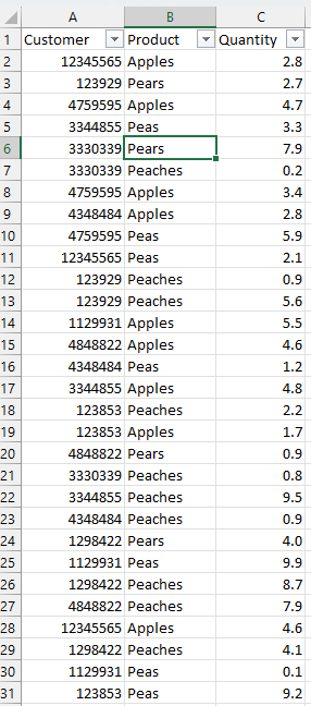
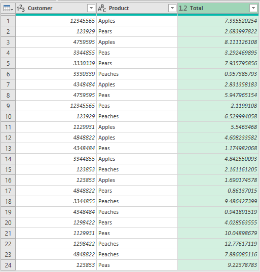
For this simple example we have some customers who have purchased different types of produce, and we want to determine which customer has purchased peas but not peaches.
Getting Data from a Range
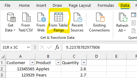
The first step in using Power Query on data within an Excel sheet is to go into the Data tab, select all of the data we wish to include, and then click “From Table / Range.”
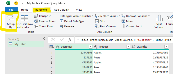
Next we will select “Group By” from the Transform menu in the Power Query interface.
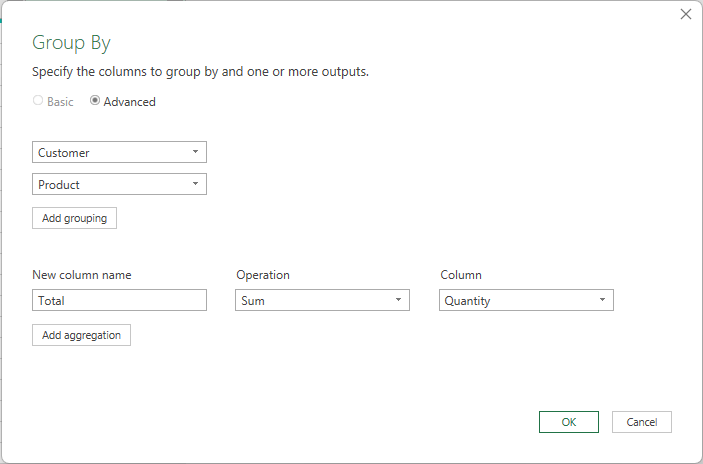
In the advanced settings it is possible to specify multiple levels of grouping. In this case we wish to group by Customer and Product and sum the quantity purchased by each customer.
There are a number of possible operations but for this example we will select a sum of the quantity column and rename the resulting column to “Total.”
This grouping operating will leave us with unique rows for Customer-Product with which we can continue our analysis.
The grouped data is displayed below showing totals for each customer and product.
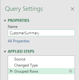
Next give the query a friendly name under “Query Settings.” We have chosen “CustomerSummary.”
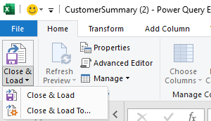
Finally under the Home tabe select “Close & Load To…” in order to save the edits and run the query.
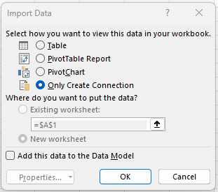
For this example we will select “Only create connection.” This is to avoid workbook clutter, but if we prefer to output intermediate steps we can create a table on a new worksheet which is the default behaviour.
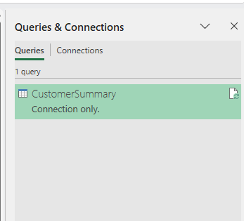
Our new Power Query now shows up in the right under “Queries & Connections.” If this does not appear it can be found under Data -> Queries & Connections.
In order to solve the example problem we will need two tables so we can perform an anti-join operation.
If you are not familiar with this terminology it just means to keep only the rows in the second table that do not have any matches in the first table. For example, of customers who purchased peas, which ones do not appear in the list of customers who bought peaches.
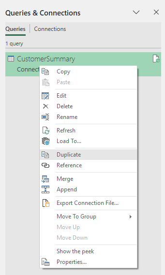
We will duplicate our query by right clicking on our query in the available connections and selecting “Duplicate.”
Let’s save our edits as above, give the query a friendly name and select “Close & Load to…” then “Create only connection.”
Note that there are two options “Duplicate” and “Reference.”
Duplicate copies the entire query with a new name, whereas reference will start a new query using the old query as the base. That can mean less load time, but sometimes it is more convenient to have separate queries in case we want to change prior steps independently.
Merge Dialog Box
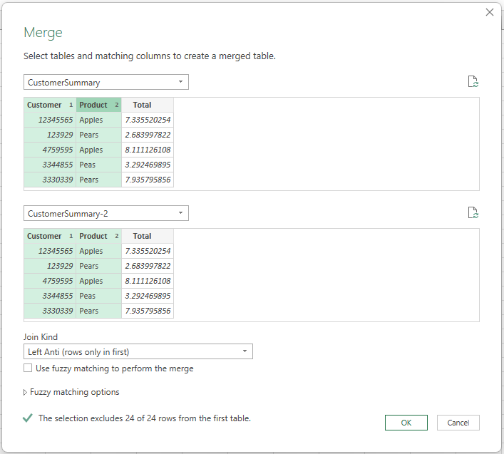
The merge dialog box is a bit complicated, the steps are:
Choose the “left” or starting query which is “CustomerSummary” in this case.
Choose the “right” or query to merge with in this case “CustomerSummary-2”
Select “Left Anti” from the menu at the bottom.
Click the Customer column in both queries until you see them highlight with a small “1” in the corner.
Hold “Control” and click Product in both queries so that a small “2” appears and they also highlight.
Holding control and clicking is how we can specify a join involving two separate columns in Power Query which is a very handy feature in some situations.
Filtering Data
The result set will appear as a new query called “Merge” which we can give a friendly name to.
Note that this result set will be empty since the lists are identical. Obviously this is not what we want, so we will need to go back and filter the lists to get the proper result.
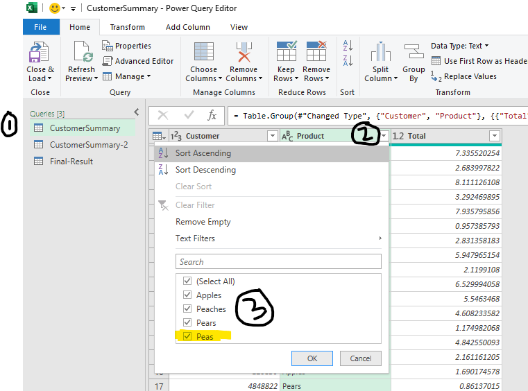
Select the first query so it becomes activated.
Select the small down arrow next two product to bring up the filter menu
Deselect everything except for Peas
Then repeat this process for the second query but selecting only Peaches.
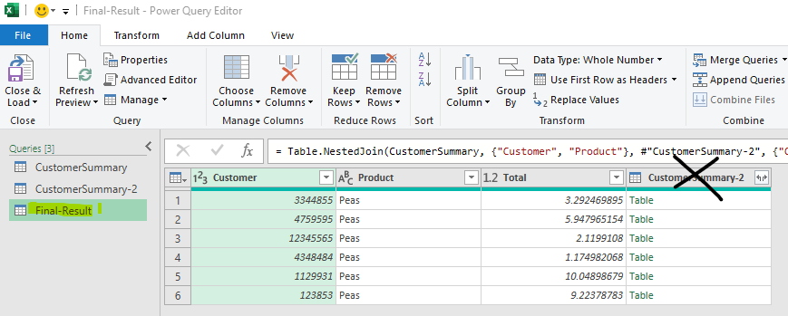
Next we click on the query in the left after giving it the friendly name of “Final-Result.”
We can also delete the right-most column by clicking on the column title and pressing the delete key.
For other types of merges we might want to expand the rows with the split arrow, but for a left anti-join these are just missing rows so we can delete the column.
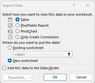
Again, let’s “Close & Load to…” but this time we will output the final result into a new sheet.
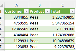
Final Result
Our final output is a table containing customers who purchased peas but did not purchase peaches. We can also see the quantity of peas these customers bought which may be relevant for further analysis.
The beautiful thing about Power Query is that these steps are reproducible, if we add more customers and produce to our original table we can simply refresh the Excel sheet and Excel will take care of the rest and generate a new listing.
We can refresh our queries by right clicking the query in the Queries & Connections pane, or simply clicking “Refresh All” in the Data tab.
Conclusion
Power Query is an excellent option for automatically the combining different sources of data.
These techniques become immensely more powerful when you combine your data with sources such as SQL databases or pull data from folders of spreadsheets that share a common form such as monthly reports from a vendor.
This article has only scratched the surface of what Power Query is capable of, it has many great features poised to efficiently streamline your Excel workflows and make them reproducible.