Minimum network flow logistics excel

Business Insights

Transportation costs are a burden on our margins and minimizing them is an effective way to improve profitability without sacrificing in other areas. Minimum Cost Network Flow Models help us get a handle on our transportation costs.

Microsoft Excel has a powerful built in optimizer called the “solver” that can make short work of these type of optimization problems with a little bit of modeling preparation.

Let’s explore how we can use Excel’s built in solver to find the optimal routing that minimizes transportation costs for a small distribution network.

Scenario

Below is a network model containing two plants (P), one warehouse (W), and two retail customers (R). There are a number of possible routes, some are bidirectional and others are unidirectional. Plants and retailers can transfer between each other, but goods only flow into and out of the warehouse.

Our goal is to minimize transportation costs given route capacity.

Results

We determine that by using the optimal routes we can minimize our shipping costs to $19,750.

Follow along below to see how we set up this model and found the solution.

Transportation Cost Matrix

The first step in setting up our logistics model is to create a matrix of nodes that can accept inflows or outflows. Based on the network above P1 (Node 1) can ship to P2 (Node 2) at a cost of $30, and W1 can ship to R1 with a cost of $10.

We grey out nodes which have no connected routes (also know as edges in network graph models).

The numbered indexes will be useful for the =INDEX() formula in Excel when we want to pull these values out and assign them to routes.

Network Flow Capacity and Costs

For simplicity we define our route capacity to be 150, and simply set all route capacities to =D13 to indicate that all routes have the same capacity. Of course if trucks assigned to the warehouse were smaller we could lower the capacity of those routes.

The network routes are simply all possible connections going both directions. Node 1 (P1) has possible destinations 2, 3, 4, and 5. This is repeated for each node.

Unit costs can be taken from the Model Transportation Matrix with the formula =INDEX($D$5:$H$9,B17,C17) or if you prefer named ranges you could give the matrix a name by using the”Name Manager” under the Formula tab. In which case it would be unnecessary to fix the rows and columns with $ (F2 Key).

This formula simply looks up the cost from the matrix given the index of the origin and destination nodes and enters it under UnitCost to indicate the route cost.

The Flow column can initially be set to all zeros or some other reasonable values. These are known as “changing cells” because solver will change these values to find the optimal solution. We colour them blue to indicate their role in the model.

Finally, total cost is =SUMPRODUCT(D17:D28,E17:E28), that is UnitCost* Flow in row 17 + UnitCost*Flow in row 18 +…+ UnitCost*Flow in the final row. SUMPRODUCT is a useful function that computes the total sum of two column arrays that are multiplied together element-wise such as SUM(Cost*Quantity).

We colour Total Cost yellow to indicate that it is the target cell, also called the objective function, to be minimized. This is the number we want solver to minimize.

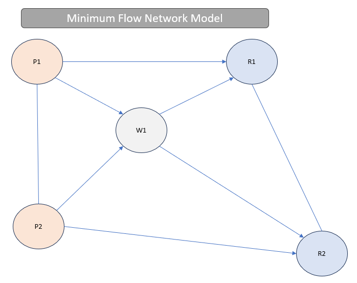
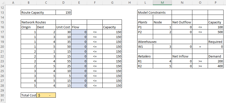
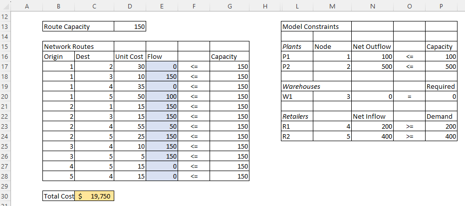
Network Flow Constraints

The most important part of any optimization problem is setting constraints. We have three types of nodes that operate in different ways.
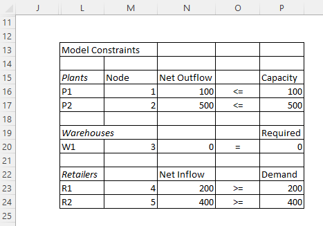
Plant Nodes

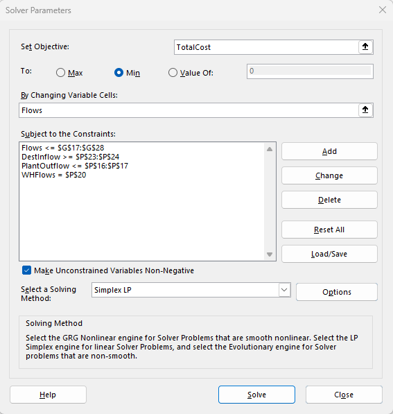
Our plant nodes (1 and 2) only have outflows subject to the capacity of the plant. In order to find the Net Outflow for Plant 1 we want to sum all of the flows originating from 1, and subtract all of the flows that have destinations at 1.

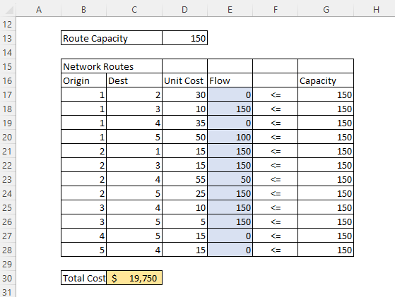
We can use the formula: =SUMIF($B$17:$B$28,M16,$E$17:$E$28)-SUMIF($C$17:$C$28,M16,$E$17:$E$28). This is the same as SUMIF(Origins, Node1, Flows) – SUMIF(Destinations, Node1, Flows) which can be set up in the name manager if you are so inclined.

Warehouse Nodes

Our warehouse only has flow through, we can think of this as a warehouse that is perpetually full and will only ship product if new product arrives to replenish the stock. It requires no capacity so this is set to zero.

The formula for warehouse is identical to the plant nodes. =SUMIF($B$17:$B$28,M20,$E$17:$E$28)-SUMIF($C$17:$C$28,M20,$E$17:$E$28)

Retailer Nodes

These nodes are our customers, and they have a total demand which matches our total capacity. If this was not the case we would not be able to solve the problem without some modifications. We may explore these in a future article.

The formula for retail nodes is the opposite of the production nodes because they only have net inflows. Net inflow must be greater than or equal to the customer demand. We can model this with SUMIF(Destinations, Node4, Flow) – SUMIF(Origins, Node4, Flow).

=SUMIF($C$17:$C$28,M23,$E$17:$E$28)-SUMIF($B$17:$B$28,M23,$E$17:$E$28)

These formulas can just be copied down to similar nodes as long as we fix columns and rows appropriately with the $ operator.

Locating Solver

The solver can be found under the data tab if it has been activated as an add-in. This add-in ships as part of modern versions of Excel but may need to be activated.

Installing Solver

If you don’t see the solver under the data tab we can install it by simply going to File > Options > Add-ins and hitting the “Go..” button for Excel Add-ins. This will present a checkbox from which to install desktop add-ins.

While you are at it the Analysis Toolpack is excellent for creating histograms and doing basic statistics in Excel.

Preparing Solver

The solver dialog is where we will set up our minimum network flow model. We have set some named ranges just to make things a bit more human readable but this is not required.

The first step is to set the objective, that is the target cell for TotalCost we coloured yellow earlier. We want to minimize this cost number so we select “min” as the type of objective.

The second step is to tell Solver where our changing cells are. Those are in our flow column and we coloured them blue earlier to indicate they are changing cells. These are the cells solver will try different values for as it searches for a solution to minimize the total cost.

Solver Constraints

Next we need to set our model constraints which we discussed above. We do this by clicking on “Add” and then entering the ranges of values and constraints in the following dialog.

They can be entered in succession by pressing “add” in the dialog and then closing when all constraints are entered.

For example, all flows must be less than or equal to the corresponding capacity we set so we enter the range of flows and the range of capacities, and specify the <= operator.

Similarly, warehouse flows must equal zero, so we specify Net Flows for the warehouse (N20) and it’s requirement of zero (P20) with the = operator.

For the plants the net outflows must be less than or equal to capacities, and for retail customers the net inflows must be greater than or equal to the demand.

Finally we select a solving method. In this case we will use the default Simplex LP which is a well known and very efficient way of solving linear programming problems.

Running Solver

Once everything has been set up we can run our model by clicking on “solve.”

We have reset all of the blue flow values to zero. This results in no total cost and no net inflows to meet customer demand. We will then run solver to find the optimal solution given our constraints.

Solution

Solver cheerfully tells us it has found a solution that satisfies our constraints, and the solution it found is $19,750 in total cost which now appears in the yellow target cell C30.

We can also see in our constraint table that net outflows from our plant nodes match capacity, our warehouse has zero net outflows, and our retailers demand has been satisfied.

Therefore, we can minimize our shipping cost in this network by using route 1:3 for 150 units, 1:5 for 100 units, and so on.

Conclusion

Excel’s solver puts powerful logistics capabilities into the hands of businesses of all sizes, it is a great option to get a handle on distribution networks.

Although modeling transportation in Excel is a lot of fun but this isn’t the end of what we can do with Minimum Cost Network Models. These models can be extended to areas such as task assignments, equipment replacement, water pipeline transport, and minimum distance problems.