Flexible Bayesian Modeling in Stan

Dustin

8 July 2024
13 min read

Introduction

This is a follow-up to Bayesian Simulation for Pricing Scenarios intended to give additional background on the Bayesian approach to data analysis, specifically with the Stan language.

Stan is a highly flexible probabilistic programming language. Although R packages like rstanarm offer very convenient interfaces for common models it may be that we don’t find a function that meets our needs, or we want to build something simpler and more performant.

While Stan excels at Bayesian simulations, it also has a number of other estimators available such as the optimizer that performs MAP (maximum a posteriori ) parameter estimation. This makes it one of the most versatile open source tools available.

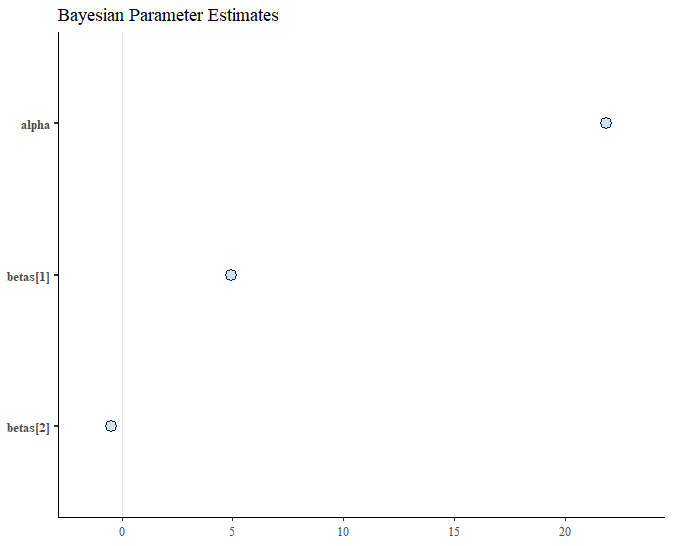
Bayesian Probability

Since our focus is primarily on business intelligence we try to avoid formulas, but it is difficult to understand what Stan is doing without at least touching on probability.

Bayes Rule famously states that the probability of(A) being true given some observed evidence (B) can be described by the following relationship.

P(A|B) = {P(B|A)P(A) \over P(B)}

This formula describes a way to update our beliefs based on evidence. For example, if we believe 50% of customers love our product, but a survey finds only 1 in 1,000 people like the product, then we would be forced to revise our beliefs with respect customer satisfaction downward.

Formula Components

The top line P(B|A) is the likelihood of seeing our observed data (evidence) given that A is true, and multiplied by our prior guess P(A) of the data generating distribution. Together, this gives us an “un-normalized” estimate of P(A|B) which is again the probability of A (a customer loving our product) given some observed evidence (the survey).

This initial estimate P(B|A)P(A) is said to be proportional to the left hand side but it isn’t useful unless we normalize it to a value between [0,1] were a probability should reside. That is until we divide it by P(B) the marginal probability. This is a thorny problem because there is often no mathematical solution to determine P(B).

Markov Chain Monte Carlo

This is where Markov Chain Monte Carlo (MCMC) comes to the rescue. As it turns out, if we take a lot of samples over the proportional version of the parameter space we can get a very good approximation of P(B) which allows us to do the division and get an answer for P(A|B) which is called the posterior probability.

Not only does this assist us in estimating the data generating mechanism, the same samples that helped us solve P(B) can be used to assess uncertainty in our estimates or provide ranges of possible outcomes.

Stan Language

Stan is at the cutting edge of MCMC samplers. It uses a type of sampling known as Hamiltonian MCMC which emulates a frictionless particle exploring the probability space. In more practical terms, it is much faster than previous incarnations of MCMC, easier to work with, and under active development.

We can also a lot with very little code. The example below demonstrates a linear regression model that takes a vector of response variables and a matrix of coefficients as data.

Stan Model File

The easiest way to create a Stan file is to select New->Stan File in R Studio. However, any text file is fine, provided it is saved with a “.stan” extension R Studio will recognize it.

As an aside, we need to ensure there is one blank line at the end of the file or a warning will trigger saying the file is incomplete. This doesn’t affect the compiler but it is a bit annoying.

/// Stan Model Code
data {
  int<lower=0> N;
  int<lower=0> K;
  vector[N] Y;
  matrix[N, K] X;
}

parameters {
  real alpha;
  vector[K] betas;
  real<lower=0> sigma;
}

model {
 // Liklihood
    target += normal_id_glm_lpdf( Y | X, alpha, betas, sigma);
}

Data Block

The data block enclosed in the {} braces tells Stan what type of data is going to be provided.

We will provide a number N that represents the number of rows in our data. K will be the number of columns in our predictor matrix. Then we define a vector Y and matrix X which we will pass in from R as our initial data.

In some implementations it would be perfectly fine to use a model matrix where the first beta is a column of 1s for the intercept, but we use alpha because that is what the normal_id_glm_lpdf function expects.

Model Block

The model block defines the likelihood and prior P(B|A)P(A). The above code tells Stan to increment the log posterior probability with values that make sense for a linear model (i.e. normal distribution) given: Response (Y), Matrix of explanatory variables (X), Intercept (alpha), coefficients (beta), and standard deviation (sigma).

The normal_id_glm_lpdf function refers to a generalized linear model with identity link which is statistics speak for linear regression. This could be programed a number of ways, but since it is a common type of model the Stan developers have kindly created a super efficient and easy to use function.

The target being incremented is the space that the sampler will explore, and this operation is vectorized but Stan understands Y[1:N] without having to be explicit.

This target format makes it easy to add priors. In this case since we did not specify any priors Stan will add non-informative priors P(A) for us. However, specifying priors can be done by simply adding to the target.

For example including target += normal_lpdf( alpha | 1000, 100) in the model block would place a prior constraint on our intercept, specifically a normal distribution with mean of 1,000 and Standard Deviation of 100.

This takes a bit of getting used to if you are familiar with BUGS language or JAGS but it is worth the effort and ends up being a much simpler way to work with the log posterior.

Parameter Block

The variables not defined in the data block are parameters which need to be estimated. Those are defined in the parameter block.

It can be helpful to read Stan code bottom to top, especially when models get larger and more exotic model blocks are used.

Simulating Data

Now that we have a Stan model let’s simulate some random sales data in R to give 500 unit volume amounts depending on price and whether the product is on-sale / promoted.

We will be using cmdstanr which is a lightweight Stan API that requires CmdStan. Instructions for the instllation in R are available at :https://mc-stan.org/cmdstanr/articles/cmdstanr.html

options(scipen = 999)
library(tidyverse)
library(cmdstanr)
library(bayesplot)

### Simulate Data
set.seed(123)
SaleStatus <- factor(sample(c("NoSale", "Sale"), 500, prob = c(0.9, 0.1), replace = T), levels = c("NoSale", "Sale"))

MakeSalesData <- function(x) {
  if(x == "Sale") {
    return(
      data.frame(SaleFlag = x, Price = rnorm(1, 5, 1))
    )
  }
  else {
    return(
      data.frame(SaleFlag = x, Price = rnorm(1, 10, 2))
    )
  }
}
set.seed(123)
Simulation <- map_df(SaleStatus, MakeSalesData) %>% 
  rowwise() %>%
  mutate(Volume = 2000 - rnorm(1, Price * 50, rgamma(1,shape = 2, rate = 1)) + 
           (as.integer(SaleFlag) - 1) * 100 * rnorm(1, 5, 1) + rnorm(1,200,50)
  ) %>% as.data.frame()

Data Preparation

Next we will transform our data by putting our response variables into a matrix “X” and change SaleFlag into an integer where 0 represents regular price and 1 represents sale price.

We will also scale our volume by 100 since the absolute value of the volume numbers are much larger than price.

Data List

CmdstanR requires a list of variables to be passed. This includes everything we defined in our data block including N for the number of elements, K for the number of predictors in our matrix, the matrix itself, and the response variable Y.

### Transform Data
X <- Simulation[,1:2]
X$SaleFlag <- as.integer(X$SaleFlag) - 1
X <- as.matrix(X)
Y <- Simulation$Volume / 100

data <- list(N = nrow(X), K = ncol(X), X = X, Y = Y)

Compile Model

Next we need to compile our model into a variable. Stan will read our code, compile it into C++ so it is super fast, and save the executable in our current working directory in case we want to run it again.

model <- cmdstan_model(stan_file = "StanGLM.stan")

Fit Model

Next we can fit our model by providing the list of data, a random seed for reproducibility, and letting Stan know to run 4 chains in parallel on 4 CPUs. We can use as many CPUs as we have chains, and generally 4 chains is a good number.

The purpose of having more than a single chain is that if all the chains come up with the same answer we can expect the sampling to be more reliable. If we only used one chain then we’d have one less sanity check on whether sampling was being done properly.

Once fit we will run a summary. Sometimes this can take a while so it’s a good practice to store the summary in a variable if we might need to use it again later.

fit <- model$sample(data = data, seed = 123, parallel_chains = 4)

MySummary <- fit$summary()
MySummary

  variable     mean     sd       q5      q95  rhat ess_bulk
  <chr>       <dbl>  <dbl>    <dbl>    <dbl> <dbl>    <dbl>
1 lp__     -436.    1.43   -439.    -435.     1.00    1433.
2 alpha      21.9   0.139    21.6     22.1    1.00    1306.
3 betas[1]    4.95  0.110     4.76     5.12   1.00    1577.
4 betas[2]   -0.487 0.0136   -0.510   -0.465  1.00    1321.
5 sigma       0.560 0.0181    0.531    0.590  1.00    2002.

This summary provides rhat values for us. If these values are approximately 1.0 then it is a good sign that our chains converged and are providing reliable estimates. If this value is 1.1 or higher then it suggests serious problems with our model.

In addition, ess_bulk tells us our effective sample size which seems reasonable for 2,000 iterations (the default setting).

We also get helpful estimates for our beta variables and intercept (alpha) that include point estimates (mean/median) and a 95% credible range. For example, our estimate of alpha ranges between 21.6 and 22.1 in terms of scaled volume.

Plotting Coefficients

We can use the Bayesplot package to easily plot our coefficients and confidence intervals. The first step is to extract our draws into a dataframe. Then we can use the mcmc_intervals function. This is a wrapper to ggplot2 so we can also change up the theme or add a title.

MyDraws <- fit$draws(format = "df")

mcmc_intervals(MyDraws[, 2:4],
               prob_outer = .95,
               prob = .8,
               point_est = "mean") +
  labs(title = "Bayesian Parameter Estimates")

Since we simulated our data with a linear function the confidence bands are too narrow to display but we can see where our point estimates land.

MAP Estimates

Although Bayesian simulations are a lot of fun, Stan has a number of other fitting algorithms. One of these is “optimize” which provides a MAP (maximum a posteriori) estimate of the parameters.

Stan’s MAP estimate is used as the default in the prophet time series model created by Facebook due to the time required to perform MCMC sampling on large time series.

MAP estimates are similar to maximum liklihood, they look for the maximum density of probability in the un-normalized log posterior P(B|A)P(A). Since it is possible to explore this space without sampling it is much faster if we don’t need to directly model uncertainty.

fit.map <- model$optimize(data = data)
fit.map$summary()

Initial log joint probability = -66846.1 
    Iter      log prob        ||dx||      ||grad||       alpha      alpha0  # evals  Notes  
      40      -433.874   7.76188e-05    0.00917981      0.6096     0.06096       73    
Optimization terminated normally:  
  Convergence detected: relative gradient magnitude is below tolerance 
Finished in  0.1 seconds.

 variable estimate
  <chr>       <dbl>
1 lp__     -434.   
2 alpha      21.9  
3 betas[1]    4.95 
4 betas[2]   -0.487
5 sigma       0.556

In this case our MAP estimates are almost indistinguishable from the Bayesian mean estimates in the above summary but they don’t lend themselves as nicely to creating credible intervals.

Credible Intervals

What makes MCMC sampling such a lovey invention, especially if we are trying to understand risk and uncertainty in the business context, is that we can use our chains to provide estimate ranges. For example, below is an estimate of expected volume outcomes given a price of $7 and promotion.

Sale7 <- (MyDraws$alpha + MyDraws$`betas[1]` * 1 + MyDraws$`betas[2]` * 7) * 100
hist(Sale7, col = "lightblue", breaks = 50, xlab = "Unit Volume", main = "Outcomes: Price $7 + Promotion")

Since we have estimated a standard deviation for each sample we could also add a random error term to our that will be similar but different for each iteration.

Although the above model accounts for uncertainty in our parameter estimates, life also has that unpredictable quality which is captured as the epsilon parameter in our model definitions.

$Y = \alpha + \beta + \epsilon$

We can simulate some randomness with the rnorm function in R using location of 0 and the standard deviation from each sample. Over the long term the mean will be the same since the expected value of epsilon is zero, but it is possible that any given event will be higher or lower than expected.

Sale7.sd <- ((MyDraws$alpha + MyDraws$`betas[1]` * 1 + MyDraws$`betas[2]` * 7) +
  rnorm(
    n = nrow(MyDraws),
    mean = 0,
    sd = MyDraws$sigma
  )) * 100

Adding an error term causes our distribution to flatten out suggesting a similar expected value, but more uncertainty over a wider range of possibilities.

This randomness can also be done in Stan if we set up a Generated Quantities block and use one of the random generator functions such as normal_rng(). Stan has a series of functions all ending in “_rng” that are helpful in quickly simulating random draws.

Since this is Stan we are also free to define almost anything we like in the Generated Quantities block. For additional details please see the Stan Reference Manual.

Production Models

CmdstanR saves our compiled models for us in “.exe” executable format so they are ready to be re-fit with new data at any time.

model2 <- cmdstan_model(stan_file = "StanGLM.stan", exe_file = "StanGLM.exe", compile = FALSE)
fit2 <- model2$sample(data = data, seed = 123, parallel_chains = 4)

Recalling Models

To recall a Stan model, we simply use the cmdstan_model function, this time specifying the “.stan” file location and the location of the compiled executable. Unless the model has changed we can also set compile = FALSE to save load time.

Conclusion

With the availability of powerful desktop computers Bayesian approaches to business analysis have gained a lot of traction as a critical skill.

Stan is an amazing program for probabilistic modeling, both in terms of its power and flexibility. Learning Stan comes with a huge payoff in being able to conduct business analysis in a way that naturally incorporates risk and uncertainty.

References

Kentaro Matsuura (2023). Bayesian Statistical Modeling with Stan, R, and Python. Springer, Singapore.
Andrew Gelman, John B. Carlin, et. al. (2013). Bayesian Data Analysis, 3rd edition.
Richard McElreath (2016) Statistical Rethinking: A Bayesian Course with Examples in R and Stan. Chapman & Hall/CRC Press.
Stan Reference Guide