Correlation between variables suggests a directional association such that an increase in one variable is associated with an increase or decrease in the other variable. For example, we might find that income is correlated with spending on luxury goods.
Partial correlation has a similar aim but it allows us to control for the effect of related variables in order to get a more precise understanding of the relationships between individual variables.
For this example we will use a customer sales and insights dataset available on Kaggle. This dataset contains customers and related sales and marketing metrics.
Loading Data
The first thing to do is load our packages, we will use the popular ppcor package for partial correlations. We will also remove non-numeric columns since we can not use these methods directly on categorical data.
Note that ppcor loads the MASS package which maks the select function in dplyr so we need to specify dplyr::select() explicitly or it will throw an error.
None of the variables in the original dataset have any correlations which would make for a boring data science article, so we will add some linear correlations to a few of the variables.
We now have LinLV (lifetime value) which is based on churn probability, and LinAOV (average order value) which is in turn based on lifetime value.
Panel Charts
A good first step in looking at correlations is to run a panel chart, the psych package has a very nice implementation.
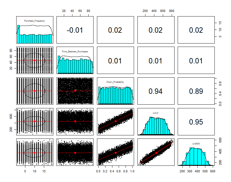
pairs.panels(SalesData)
As expected churn probability correlates highly with lifetime value and average order value.
We can see that these variables follow a normal distribution and that the data appears linear. This is important for Pearson correlation but less so for Spearman correlation which is better at detecting non-linear relationships.
Other variables look random. They appear to have uniform distributions and no relation to other variables.
Correlation
Since relationships look linear we will use Pearson correlation to explore these relationships.
Next we will explore partial correlations between these variables with the pcor function. The output is quite large so we will extract the relevant parts for brevity.
The estimates in the top of the readout tell us much more than a simple correlation matrix. Lifetime value has a much lower correlation to churn probability holding the other variables constant.
Similarly, average order value has a lower correlation to lifetime value and almost no correlation to churn probability while holding other variables constant. This is a very different result than the one we obtained with a basic correlation matrix.
P-values are also conveniently available to assess whether correlations are significant, in this case they are.
We can also test specific pairs variables with pcor.test. We look at the correlation of vector x with vector y, while holding a third vector z constant. This gives a more reliable, as in repeatable, estimate than we would get by controlling for many variables at the same time.
pcor.test(
x = SalesData$Churn_Probability,
y = SalesData$LinAOV,
z = SalesData$LinLV)
      estimate   p.value  statistic     n gp  Method
1 0.0008510263 0.9321916 0.08508989 10000  1 pearson
We obtain a similar result to the partial correlation matrix. The correlation between churn probability and average order value is not significant after controlling for lifetime value. In other words, lifetime value is more likely to be causing the variation.
This makes sense because when creating the data we built lifetime value from churn probability, and then based average order value on lifetime value.
Semi Partial Correlation
The pcor package also has a function for semi-partial correlations. In partial correlation the third variable is held constant for both X and Y. With semi-partial this becomes X or Y, so the third variable is held constant for X or Y, but not both at the same time.
To investigate semi-partial correlations we can use spcor or spcor.test which operate identically to the pcor functions.
Using semi-partial correlation the correlation of both LinLV and LinAOV are lower.
In addition, the correlations are not longer symmetric. LinLV correlates 0.293 with churn probability, but churn probability correlates 0.204 with LinLV.
This directionality can be useful, the X variables appear on the right, and the Y variables in the columns. Therefore, we can see that churn probability does a better job predicting LinLV than vice-versa which provides clues on causality.
Again, this makes sense because we originally built LinLV off churn probabilities.
Conclusion
Partial correlations can help unmask more precise relationships between variables and provide clues on the direction of causal effects. The pcor package makes understanding these relationships a breeze.