Life is all about choices, and we can use logistic regression to understand the reasons behind customer decisions. Better understanding the reasons behind the choices our customers make is helpful in improving our pricing and promotional strategies.
Let’s explore how we can use binomial regression to identify important factors in customer decisions related to drink purchases.
Scenario
Let’s assume we are operating a very posh cold beverage stand and customers can choose between a chocolate milkshake or an energetic fruit smoothie. We want to understand what factors are related to customers choosing the smoothie over the milkshake.
Results
We determine that each dollar of price decreases the liklihood of smoothie purchase by 17%, whereas increasing days of the week increase the odds by 24%.
Follow along below in R Studio to see how we arrived at these insights.
Generating Data
For this analysis we will generate some sales data where a choice of 1 indicates that the customer choose the smoothie, and 0 indicates they choose a high end milkshake.
The binomial distribution models the probability of getting some number of successes in some number of trials. In our case it is how many times the product is successfully chosen by a customer given the total number of products selected in the category.
Generalized Linear Models
The binomial model is a Generalized Linear Model (GLM). These models are similar to linear regression, or more specifically linear regression is just a type of GLM.
All GLMs are based on the familiar combination of linear predictors with slopes, coefficients, and an intercept.
Y = \alpha + \beta\scriptscriptstyle 1 \normalsize X \scriptscriptstyle1 \normalsize + \beta\scriptscriptstyle2 \normalsize X\scriptscriptstyle 2 \normalsize… + \epsilon
GLMs have a “link” function which in the case of the binomial model is most often the logit (log odds) function. This function is the canonical link function for binomial models.
logit(P) = \ln({P \over 1-P})
Link functions relate the linear combination of predictors to the mean of the intended probability distribution. In the case of the binomial model the mean is np, the number of trials multiplied by the probability of success.
When we transform our response variable by the logit function and run the linear regression, we will end up with log coefficients, representing log-odds, related to a binomial outcome with mean np.
Logistic Regression
To run a logistic regression in R we specify our response “Choice” and the predictors we wish to include on the right hand side. The only difference from ordinary least squares is the inclusion of the family as “binomial.”
We can specify a link function, but this family defaults to the canonical logit link which is exactly what we need for a logistic regression.
glm.mod <- glm(Choice ~ Price + Sex + Day + Income,
family = "binomial", data = Data)
summary(glm.mod)
Call:
glm(formula = Choice ~ Price + Sex + Day + Income, family = "binomial",
    data = Data)

Coefficients:
             Estimate Std. Error z value Pr(>|z|)
(Intercept) -0.142800   0.347692  -0.411    0.681
Price       -0.195794   0.025546  -7.664 1.80e-14 ***
Sex          0.200020   0.168038   1.190    0.234
Day          0.210938   0.037335   5.650 1.61e-08 ***
Income       0.020870   0.002345   8.900  < 2e-16 ***
---
Signif. codes:  0 ‘***’ 0.001 ‘**’ 0.01 ‘*’ 0.05 ‘.’ 0.1 ‘ ’ 1

(Dispersion parameter for binomial family taken to be 1)

    Null deviance: 1320.0  on 999  degrees of freedom
Residual deviance: 1144.6  on 995  degrees of freedom
AIC: 1154.6

Number of Fisher Scoring iterations: 4
Interpretation
We have the familiar linear coefficients, the only difference is that they represent log odds. However, we can immediately see that price has a negative relationship with product choice, income and day have positive relationships, and sex does not have a significant relationship.
Overdispersion
Another nuance of generalized linear models is that they have dispersion parameters. In the case of the binomial model dispersion is assumed to be 1.0 which the output kindly indicates.
One way to check for overdispersion is to compare the residual deviance to the residual degrees of freedom. In this mode the residual deviance (1,144) is slightly higher than 996 which indicates that some overdispersion is likely present.
This is not a good thing as it can impact the standard error estimates, which in turn determine whether or not a predictor is statistically significant. In this case our overdispersion is not massive, but still less than ideal.
We can also run ANOVA on the model which tells us a similar story.
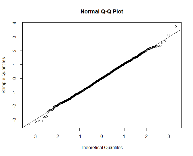
Another important diagnostic is the qq plot which helps us determine if our data are normally distributed, which is one of the assumptions of generalized linear models.
qres <- qresid(glm.mod)
qqnorm(qres)
abline(0,1)
The fitted model looks not quite normal in the right tail which could affect our estimates. Like the overdispersion level, it’s not ideal but may not be the end of the world depending what level of precision we are looking for.
One way to correct this issue might be to try a log transformation on some of the predictors, but we will leave it as is for now.
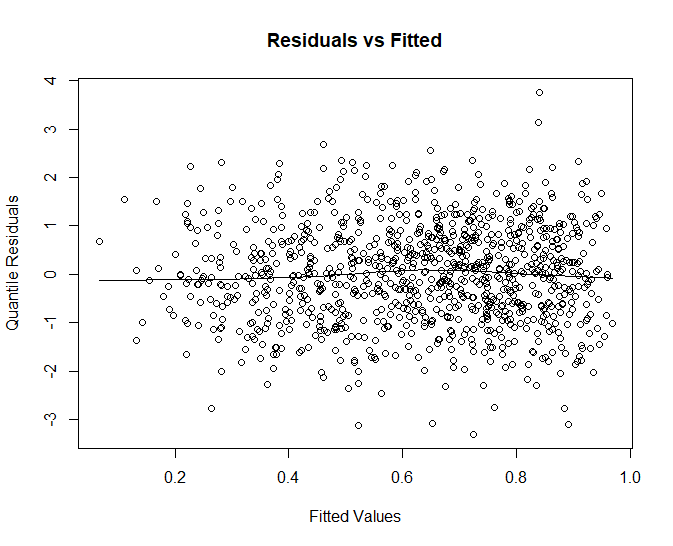
Finally, we can check our residual plot to make sure there are no obvious patterns. Since this is a glm we will plot out the quantile residuals. These are normalized residuals.
scatter.smooth(qres ~ fitted(glm.mod), main = "Residuals vs Fitted",
               xlab = "Fitted Values", ylab = "Quantile Residuals")
Like our other measures the residuals look a bit off, generally they have a nice random cloud shape, but there are what appears to be some short runs that form patterns, this might indicate some auto correlation or lack of independence between observed values.
Influential Observations
Next we can check for influential observations that may be be causing overdispersion or exerting too much leverage on the fit of our model. The influence.measures function can help run a variety of tests on each component.
The model generally checks out, the coefficients are fine but there are a influential observations related to covariance. This is not going to have a major effect on our model, we would be more concerned about influential predictors.
Cook’s Distance
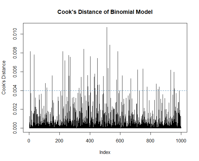
Another way to identify influential observations that are potential outliers is Cook’s distance. This is a measure describing the leverage a data point has on the model.
glm.cd <- cooks.distance(glm.mod)
plot(glm.cd, type = "h", ylab = "Cook's Distance", main = "Cook's Distance of Binomial Model")
abline(h = 4/nrow(Data), lty = 2, col = "steelblue") # add cutoff line
Data[which.max(glm.cd),]
   Sex    Price Day Income      Prob Choice
512   0 18.49668   3     50 0.1191718      1
Observation 512 which is a high price on Wednesday from a low income customer is our most influential observation. We might want to consider whether the product price was correctly recorded that day, but first we will look at the overall context.
A common rule of thumb is that influential observations have a Cook’s distance that is above 4/n, with n being the number of rows in the dataset. Influential observations are not always bad, they can be real values generated by the process we are investigating.
In this case, none of the Cook’s Distances are near 1, or even 0.1 so we won’t concern ourselves with investigating these values. We might get a better fit by removing the extreme values, but our model would then be unable to capture the process that generated them.
Model Fit (Pseudo R2)
Although there is no R Squared value for logistic regression we can calculate a Pseudo R2 value with help from the DescTools package. This is 1 minus the log likelihood of the fitted model divided by the log likelihood of a model containing only an intercept term.
library(DescTools)
PseudoR2(glm.mod)
 McFadden
0.1328923
Our predictors explain about 13% of the variation in our choice response which suggests we are missing some important predictors or there is a sizable random component that can not be accounted for.
Removing Insignificant Terms
Since Sex is not significant we will want to remove it to keep the model parsimonious and recheck our diagnostics.
glm.mod <- glm(Choice ~ Price + Day + Income, family = "binomial", data = Data)
summary(glm.mod)
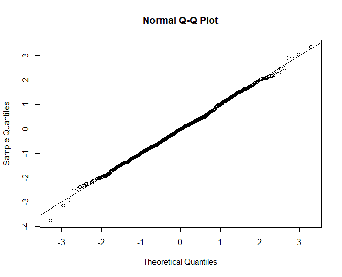
qres <- qresid(glm.mod)
qqnorm(qres)
abline(0,1)
Call:
glm(formula = Choice ~ Price + Day + Income, family = "quasibinomial",
    data = Data)

Coefficients:
             Estimate Std. Error t value Pr(>|t|)
(Intercept) -0.090039   0.348945  -0.258    0.796
Price       -0.196482   0.025871  -7.595 7.09e-14 ***
Day          0.211627   0.037773   5.603 2.73e-08 ***
Income       0.020881   0.002374   8.796  < 2e-16 ***
---
Signif. codes:  0 ‘***’ 0.001 ‘**’ 0.01 ‘*’ 0.05 ‘.’ 0.1 ‘ ’ 1

(Dispersion parameter for quasibinomial family taken to be 1.024954)

    Null deviance: 1320  on 999  degrees of freedom
Residual deviance: 1146  on 996  degrees of freedom
AIC: NA

Number of Fisher Scoring iterations: 4
The qq plot looks much more normal, only a small bit of skewness remains in the right tail.
Revisiting Overdispersion
Recall that we found some overdispersion in our model. One way to correct the potential issues with our standard errors is to run a quasi-binomial model. This will give the same coefficients but larger standard errors since it allows our dispersion parameter to scale.
To fit this type of model we just have to specify “quasibinomial” as the family.
glm.mod <- glm(Choice ~ Price + Day + Income,
family = "quasibinomial", data = Data)
summary(glm.mod)
Call:
glm(formula = Choice ~ Price + Day + Income, family = "quasibinomial",
    data = Data)

Coefficients:
             Estimate Std. Error t value Pr(>|t|)
(Intercept) -0.090039   0.348945  -0.258    0.796
Price       -0.196482   0.025871  -7.595 7.09e-14 ***
Day          0.211627   0.037773   5.603 2.73e-08 ***
Income       0.020881   0.002374   8.796  < 2e-16 ***
---
Signif. codes:  0 ‘***’ 0.001 ‘**’ 0.01 ‘*’ 0.05 ‘.’ 0.1 ‘ ’ 1

(Dispersion parameter for quasibinomial family taken to be 1.024954)

    Null deviance: 1320  on 999  degrees of freedom
Residual deviance: 1146  on 996  degrees of freedom
AIC: NA

Number of Fisher Scoring iterations: 4

>
With the Quasi-Binomial model our standard errors are slightly larger, but our predictors are still significant. We can see that the scaled dispersion parameter is 1.024, not ideal but not large enough to be overly concerned about for business analysis.
Interpretation
Since log odds are not an easy thing to communicate, we can exponentiate our coefficients to determine the odds ratio, and then subtract 1. This provides us with the percentage increase in odds per unit of predictor.
exp(coef(glm.mod)) - 1
(Intercept)       Price         Day      Income
-0.08610427 -0.17838360  0.23568631  0.02110047
We can say that one dollar in price decreases the odds of purchase by about 17%, and income level increases odds of purchase by about 2%. These become rough estimates beyond one unit of change.
Since our values are not on a linear scale we can’t simply add them together. If we want to understand the increase in purchase odds on a Saturday (Day = 6) we have to calculate on the log scale and then exponentiate.
exp(coef(glm.mod)["Day"] * 6) - 1
     Day
2.559995
This tells us that odds of purchase on a Saturday increase by about 255% compared to a Sunday (Day = 0).
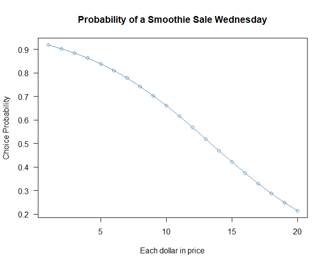
Plotting Price Changes
We can also plot out price changes for a typical customer on Wednesday by passing new data to the predict function.
NewData <- data.frame(
  Day = 2,
  Income = 110,
  Price = 1:20
)

plot(predict(glm.mod, newdata = NewData, type = "response"),
     xlab = "Each dollar in price",
     ylab = "Choice Probability",
     main = "Probability of a Smoothie Sale Tuesday",
     col = "steelblue",
     pch = 1,
     type = "o",
     las = 1)
As the price passes around $5 the probability of a purchase begins to decline more rapidly.
Odds to Probability
We can also communicate results in terms of probabilities with the inverse logit function which is defined above. The mapping is non-linear so it can be helpful to focus on how a change in log odds impacts the probability of the event.
We will consider a change in price from $5.99 to $9.99 on a Wednesday given a customer with 100K in income.
We can say that the probability of purchasing a smoothie given the price declines from 77% to 61% given the specific change in price.
Marketing Strategy
Though the exercise we have determined that Sex is not a relevant factor for targeting our smoothie promotions. Further, that some days of the week are better for smoothie sales, if we wanted to build up our clientele we might try some discounting on Wednesday, or if we wanted to leverage the seasonality we might run ads on Saturday.
When considering our pricing strategy we can also consider what it would cost to switch more customers over to smoothies, especially if they cost less to produce. That could be modeled out considering lost revenue on existing customers compared to the marginal increase for customers who switch.
Conclusion
Understanding how customers make choices and which customers make choices is critical information for both strategic and tactical decision making. Logistic regression models are a great choice to shed light on the factors behind the decisions our customers are making.
References
Chapmen, C.; McDonnell Feit, E. R for Marketing Research and Analytics; Springer, 2015.
Dunn, P.; Smyth, P. Generalized Linear Models With Examples in R; Springer, 2018.
Gelman A.; Hill J. Data Analysis Using Regression and Multilevel/Hierarchial Models; Cambridge, 2007.