Negative Binomial Real Estate Sales

Dustin

17 May 2024
6 min read

Business Insights

Risk perception is not something most people are especially good at. It can depend on personal biases, or even mood. People often over-estimate their own ability in this area. Fortunately, we can lean on probability distributions to put things into perspective and this can help us make more informed decisions.

Let’s explore how we can we evaluate a business proposal using a negative binomial model and some past performance data.

Our Scenario

A junior real estate agent receives a fixed salary of $50,000 and sells property on our behalf. When she makes a sale we receive $4000 and we like to keep 50% for profit and overhead. Last year she sold 25 homes in 365 days. Having more experience, she is promising an optimistic 50 sales and asking for a $100,000 salary.

Data Model

A negative binomial model helps us understand the probability of some number of successes happening over some number of failures. Such as selling 2 houses over 30 days.

Results

We decide against the offer and make a fair counter-proposal of $70,000 taking into account a 50% increase in sales skills. To find out how we arrived at this proposal follow along below.

Simulate Data

First let’s simulate one year of data with zero as a failure and the number of homes sold as a positive integer.

options(scipen = 999)
library(tidyverse)

set.seed(93)
HomeSales <- rbinom(365, rpois(365, 3), 0.02)
HomeSales

sum(HomeSales >= 1) # Homes Sold per Year

[1] 0 0 0 0 0 0 0 0 0 0 0 0 0 0 0 0 0 0 0 0 0 0 0 1 0 0 0 0 1 0 0 0 0 0 0 0 1 0 0 0
<...>

Next let’s explore the data identifying the number of successes (25), and the number of failures. For the failures we are interested in understanding how many occur before a success, and recall if there is a success it can be more than one. To do this we identify non-zero values and difference their positions as a convenient way to count the zeros in between.

## Calculate Failures Before Success
TotalFailures <- c(which(HomeSales >= 1)[1], diff(which(HomeSales >= 1)))
TotalFailures


## Calculate Vector of Success
TotalSuccess <- HomeSales[which(HomeSales >= 1)]
TotalSuccess


> TotalFailures
 [1] 24  5  8 20 47  4  5 12  2 12 14  1 12  2  2  6  6 10  1 17 11 21 87 16
> TotalSuccess
 [1] 1 1 1 1 2 1 1 1 1 1 1 1 1 1 1 1 1 1 1 1 1 1 1 1

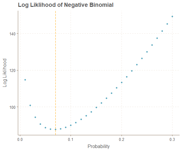
Next we want to calculate the maximum likelihood estimate because that will give us the negative binomial probability to use for our distribution. This is the probability that is most likely given the data we have available.

We write a simple function that takes two vectors of the same length to represent 24 failures 1 success, 4 failures one success, and so on. We ignore the string of failures at the end when the year runs out.

We look for the minimum log likelihood value for the probability and minimize it. Recall for negative binomial we need to use “dnbinom,” if you mistakenly type “dbinom” you will end up with strange results, which is not what we want.

### Maximum Likelihood Estimation

lh <- function(p) {
  -sum(dnbinom(TotalFailures,TotalSuccess, prob=p, log = T))
}

Phat <- nlm(lh, .001, stepmax = .05, print.level = 1)
Phat$estimate

iteration = 7
Parameter:
[1] 0.06756707
Function Value
[1] 87.63019
Gradient:
[1] -2.088996e-06

Relative gradient close to zero.
Current iterate is probably solution.

> Phat$estimate
[1] 0.06756707

Let’s see if we get the same result manually calculating these values to ensure our function works properly. We will use a grid search of possible values between 0.01 and 0.30 and put these results into a dataframe.

## Compute Log Liklihood
LogLik <- vector()
p <- seq(0.01, 0.30, by = 0.01)
for(i in 1:length(p)){
  LogLik[i] <- -sum(dnbinom(TotalFailures, TotalSuccess, prob = p[i], log = TRUE))
}
LogLik
LogData <- data.frame(
  Prob = p,
  LL = LogLik
)

#### 

ggplot(LogData, aes(Prob, LL)) + geom_point() + labs(
  x = "Probability", y="Log Liklihood", title = "Log Liklihood of Negative Binomial"
) + geom_vline(xintercept = LogData[which.min(LogData$LL),1], lty=5, col="orange")

LogData[1:10,]

> LogData[1:10,]
   Prob        LL
1  0.01 114.72542
2  0.02 100.89931
3  0.03  94.30117
4  0.04  90.68428
5  0.05  88.71829
6  0.06  87.81108
7  0.07  87.64719
8  0.08  88.03867
9  0.09  88.86462
10 0.10  90.04280

The minimum value occurs between 6% and 7% so our minimization function checks out. We could have also divided 25/365 and got a reasonable estimate.

Now let’s move onto checking out the distribution. We will turn things around a bit vectorizing the number of successes in 364 days since it makes more sense for this problem.

### Distribution
x <- seq(1, 100, by = 1)
y <- dnbinom(364, size = x, prob = Phat$estimate)
MaxProb <- x[which.max(y)]
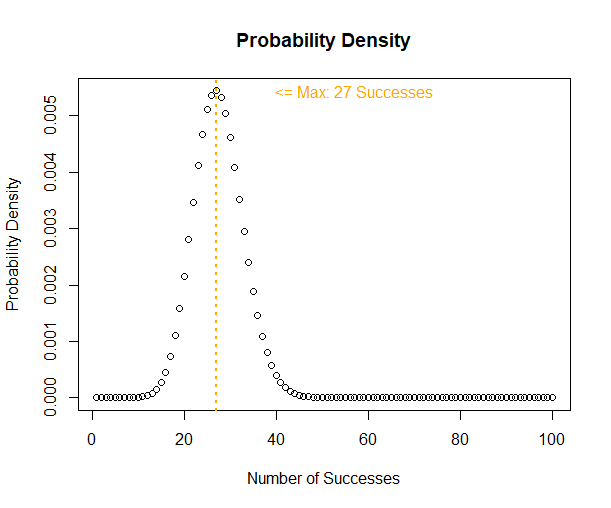
plot(y, main = "Probability Density", ylab = "Probability Density", xlab = "Number of Successes") 
abline(v=MaxProb, col="orange", lty=3, lwd = 2)
text(x = MaxProb+30, y = max(y), paste0("<= Max: ", MaxProb, " Successes"), col="orange")

The maximum value occurs at 27 and and past 40 things start looking extremely unlikely. Next let’s check the cumulative probability to see how achievable the proposal is compared to the existing agreement.

### Cumulative Probability

pnbinom(365, 25, prob = Phat$estimate)
pnbinom(365, 50, prob = Phat$estimate)

> pnbinom(365, 25, prob = Phat$estimate)
[1] 0.636078
> pnbinom(365, 50, prob = Phat$estimate)
[1] 0.00006138905

Selling 25 homes in 365 days is very achievable at a 63% probability. However, selling 50 looks extremely unlikely. However our salesperson has improved her skills over the past year and want to make a counter offer that is fair and objective.

Let’s run a simulation to see if counter-offering a salary based on selling 35 homes given that we believe our junior salesperson has improved her closing skills by 50% over the past year.

### Simulation

set.seed(93)
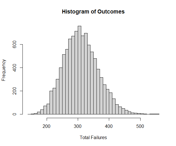
sim <- rnbinom(10000, 35, prob = Phat$estimate * 1.5)
hist(sim, breaks = 50, main = "Histogram of Outcomes", xlab = "Total Failures")
mean(sim)
quantile(sim, p = seq(.1,1, by = 0.05))

> quantile(sim, p = seq(.1,1, by = 0.05))
 10%  15%  20%  25%  30%  35%  40%  45%  50%  55%  60%  65%  70%  75%  80%  85%  
 241  254  263  272  279  287  294  301  308  315  322  329  337  346  356  368

Our intuition seems reasonable, continuing with the 60% probability of success she enjoyed last year we can expect to see roughly 322 failures before 35 successes (~365). This is to say 60% of our simulated runs show her meeting the goal of 35 sales within one year.

So we can calculate a fair $70,000 counter offer as follows since we pay $2,000 per sale. (We could write a function to find this value if we lacked subject expertise or needed more precision.)

Deals <- 35
Salary <- 2000 * Deals
Salary
>70000

In conclusion, we’ve seen that the negative binomial is helpful when dealing with multiple successes within a number of failures. As an added bonus we can say that our process is fair based on past performance after taking into account future performance.

We might improve this simple example by adding some probabilities for the number of listings available or seasonal differences which might be the subject of a future post on Bayesian networks.

References

Matloff, N. Probability and Statistics for Data Science. Chapman Hall / CRC (2019).