It can be difficult to tell whether featuring a product in advertising is contributing to sales because promotion often occurs in parallel with price breaks. It is even more difficult to quantify the relative contributions and determine an optimal strategy for advertised price.
Let’s explore how we can use Poisson regression to help us understand whether advertising or price is contributing more to our weekly sales.
Solution Range
Possibilities for price range from advertising with no price break to the other extreme of giving a price break with no advertising.
Data Required
To run analysis we will need data that coincides with the promotional cadence including whether the item was being promoted and what the average price was.
Results
We will see that price changes the rate of unit turnover by about 18% per dollar, while promoting the product in the flyer increases the rate by 62%.
Follow along below to see how we arrived at this conclusion. In a later article we will use the results to determine an optimal promotional price.
Simulated Data
First we will simulate some weekly sales data and try to recover the results with Poisson regression.
## Which weeks did promotion happen
PromoWeeks <- c(2,5,20,25,34)

## Simulate 52 Weeks of data with increasing pricing and random sale pricing
set.seed(93)

FlyerData <- data.frame(
  Week = seq(1,52),
  Flyer = rep(0,52),
  Price = c(rep(15.99,20), rep(16.99, 30), rep(17.99,2))
)

FlyerData[PromoWeeks, ] <- data.frame(
  Week = PromoWeeks,
  Flyer = rep(1, length(PromoWeeks)),
  Price = sample(c(11.99, 12.99, 13.99), length(PromoWeeks), replace = T)
)

FlyerData$Quantity <-
  round(rnorm(
    52,
    mean = 1000 + (-50 * FlyerData$Price) +
      (1 * FlyerData$Flyer * rnorm(52, 200, 25)),
    sd = 25
  ),0)

## What Were our sales
FlyerData$Sales <- round(FlyerData$Quantity * FlyerData$Price,0)

## Normally we see 2000 customers, but when promotion happens we add 100
FlyerData$Customers <- round(rnorm(52,2000, 150),0) + (FlyerData$Flyer * round(rnorm(52,100, 10)))
FlyerData$Purchase <- FlyerData$Quantity / FlyerData$Customers
Plotting Data
Let’s quickly plot our data. This looks like real sales data, we have some variation around the primary price points, and what look like outliers in the top left which suggest weeks with both promotion and price.
plot(FlyerData$Price, FlyerData$Sales,
     main = "Weekly Sales by Average Price",
     xlab = "Price", ylab = "Weekly Sales")
Poisson Model
Poisson models are a good choice for count data but they assume that the variance of the data is the same as the mean which is rarely the case with sales data. Let’s see what happens if we run a regular Poisson model.
glm.mod <- glm(Quantity ~ Price + Flyer, family = "poisson", FlyerData)
summary(glm.mod)

deviance(glm.mod)
sum(resid(glm.mod, type = "pearson")^2)
Call:
glm(formula = Quantity ~ Price + Flyer, family = "poisson", data = FlyerData)

Coefficients:
            Estimate Std. Error z value            Pr(>|z|)
(Intercept)  8.37099    0.23235  36.028 <0.0000000000000002 ***
Price       -0.19467    0.01397 -13.934 <0.0000000000000002 ***
Flyer        0.48186    0.05514   8.738 <0.0000000000000002 ***
---
Signif. codes:  0 ‘***’ 0.001 ‘**’ 0.01 ‘*’ 0.05 ‘.’ 0.1 ‘ ’ 1

(Dispersion parameter for poisson family taken to be 1)

    Null deviance: 2602.1  on 51  degrees of freedom
Residual deviance:  152.3  on 49  degrees of freedom
AIC: 525.69

Number of Fisher Scoring iterations: 4
Our residual deviance (152) is over 3 times larger than the model degrees of freedom (49) suggesting that over dispersion is an issue. Over-dispersion can lead to a model finding statistically significant results when they do not exist, basically causing the model to hallucinate. This is not what we want, so other options are a negative binomial model, or a Quasi-Poisson. We will try the latter and see if this gets us results.
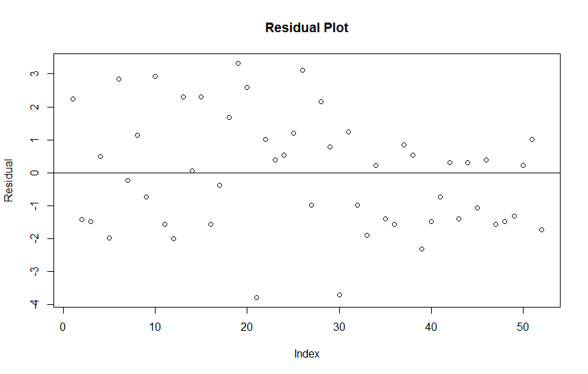
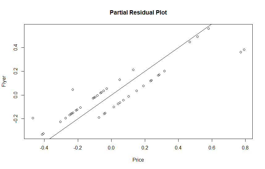
Next we run some diagnostic plots to see if we have any issues with the basic model assumptions. The Residuals should appear random, not having any obvious patterns, the partial residual plots should be linear. We will also look at the summary and exponentiated coefficients.
## Plot residuals/partial residuals and check that output is linear
plot(resid(glm.mod), main = "Residual Plot", ylab="Residual")
abline(0,0)
plot(resid(glm.mod, type = "partial"), main = "Partial Residual Plot")
abline(0,1)

summary(glm.mod)
exp(coef(glm.mod))
Call:
glm(formula = Quantity ~ Price + Flyer, family = "quasipoisson",
    data = FlyerData)

Coefficients:
            Estimate Std. Error t value             Pr(>|t|)
(Intercept)  8.37099    0.40946  20.444 < 0.0000000000000002 ***
Price       -0.19467    0.02462  -7.907       0.000000000265 ***
Flyer        0.48186    0.09718   4.959       0.000008917815 ***
---
Signif. codes:  0 ‘***’ 0.001 ‘**’ 0.01 ‘*’ 0.05 ‘.’ 0.1 ‘ ’ 1

(Dispersion parameter for quasipoisson family taken to be 3.105599)

    Null deviance: 2602.1  on 51  degrees of freedom
Residual deviance:  152.3  on 49  degrees of freedom
AIC: NA

Number of Fisher Scoring iterations: 4

> exp(coef(glm.mod))
 (Intercept)        Price        Flyer
4319.9131428    0.8231067    1.6190843
>
Results
Increasing or decreasing price changes the rate of unit turnover by about 18% per dollar, while promoting the product in the flyer increases the rate of weekly turnover by about 62%
As it turns out price and promotion also have an interaction effect because they work together, but that may be a subject for another post where we work on optimization.
Conclusion
Now that we understand the relationship between unit turnover, price, and flyer promotion, we want to run an optimization that includes our unit cost and cost the promotion to try and determine how to maximize our gross margin.
References
Dunn, Peter; Smyth, Gordon. Generalized Linear Models With Examples in R. Springer, 2018.