CarMod <- select(CarPrices, carwidth, citympg, enginesize, cylindernumber, horsepower, carlength, highwaympg,
aspiration, wheelbase, price) %>% mutate(cylindernumber = case_when(
cylindernumber == "one" ~ 1,
cylindernumber == "two" ~ 2,
cylindernumber == "three" ~ 3,
cylindernumber == "four" ~ 4,
cylindernumber == "five" ~ 5,
cylindernumber == "six" ~ 6,
cylindernumber == "seven" ~ 7,
cylindernumber == "eight" ~ 8,
cylindernumber == "twelve" ~ 12
))
CarMod <- mutate(CarMod, price = as.integer(round(price)/1000))
dists <- list(
carwidth = "gaussian",
citympg = "poisson",
enginesize = "gaussian",
cylindernumber = "poisson",
horsepower = "poisson",
carlength = "gaussian",
highwaympg = "poisson",
aspiration = "binomial",
wheelbase = "gaussian",
price = "poisson"
)
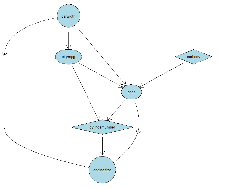
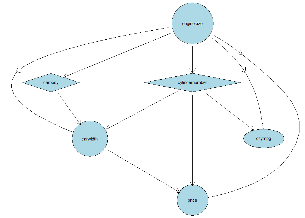
### Network Bans
ban.mat <- matrix(0, nrow = 10, ncol = 10, dimnames = list(names(dists), names(dists)))
ban.mat[,"price"] <- 1
ban.mat["carlength", c("highwaympg", "citympg")] <- 1
ban.mat["horsepower", c("citympg", "highwaympg")] <- 1
### Retained Edges
### X depends on Y
retain.mat <- matrix(0, nrow = 10, ncol = 10, dimnames = list(names(dists), names(dists)))
retain.mat["citympg", c("enginesize")] <- 1
retain.mat["cylindernumber", c("enginesize")] <- 1