Business Insights
Services are very different from products. They are inherently risky for customers because they are produced and consumed at the same time.
Customers rarely complain but will stop showing up if they are unhappy so keeping a pulse our service quality is essential.
Let’s explore how we can use Bayesian Network models to understand what factors influence a customer tip at a hair salon and then use the tip to determine if ongoing service levels are up to our standards.
Data Required
The tip is our evidence of customer satisfaction and we want to use the amount to determine if haircut quality was satisfactory. We ask our receptionist to record the tip values and ambiance of the salon for a number of months and then assign a simple rating to each stylist using our own experience.
Results
An average stylist who receives a tip between $5 and $10 is 49% likely to have delivered exceptional service. Follow along with the example below to see how we arrived at this conclusion.
Bayesian Services Model
Product marketing typically involves managing the 4 Ps (Price, Packaging, Place, Promotion).
Services marketing extends this idea with more Ps for People, Process, and Physical Evidence. Since services are intangible customers look for evidence of the service (a nice haircut). Service quality also depends on the process (wait time), and is of course inseparable from the people delivering it (friendly).
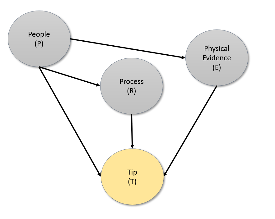
In our example we create a model where Tip depends on all three Ps. Process also depends on the skill of our people, and quality of work (Physical Evidence) similarly depends on those delivering it.

Simulate Data
All analysis starts with data to get started. We use a t-distribution around $5 to generate tip amounts and then use that result to randomly assign values to the categorical variables for People, Process, and Evidence.
As an aside, the bn.fit function complains about tibbles so at the end we transform it into an ordinary data.frame.
options(scipen = 999)
library(tidyverse)
library(bnlearn)
library(Rgraphviz)

## Simulate Data
set.seed(123)
Tips <- rt(1000,5) * 5 + 5 # Random T variable with scale = 5 and location = $5
Tips <- data.frame(Tips = round(ifelse(Tips < 0, 0, Tips),2))

Service <- function(People) {

    case_when(
      People == "Great" ~ sample(c("Great", "Average", "Poor"), 1, prob = c(0.7, 0.2, 0.1)),
      People == "Average" ~ sample(c("Great", "Average", "Poor"), 1, prob = c(0.1, 0.7, 0.1)),
      People == "Poor" ~ sample(c("Great", "Average", "Poor"), 1, prob = c(0.7, 0.2, 0.1)),
    )
}

Tips <- rowwise(Tips) %>% mutate(

  Evidence = factor(case_when(
    Tips == 0 ~ sample(c("Happy", "Neutral", "Unhappy"), 1, prob = c(0.1, 0.1, 0.8)),
    Tips > 0 & Tips <= 5 ~ sample(c("Happy", "Neutral", "Unhappy"), 1, prob = c(0.1, 0.8, 0.1)),
    Tips > 5 ~ sample(c("Happy", "Neutral", "Unhappy"), 1, prob = c(0.8, 0.1, 0.1)),
  )),
  People = factor(case_when(
    Tips == 0 ~ sample(c("Great", "Average", "Poor"), 1, prob = c(0.1, 0.1, 0.8)),
    Tips > 0 & Tips <= 5 ~ sample(c("Great", "Average", "Poor"), 1, prob = c(0.1, 0.8, 0.1)),
    Tips > 5 ~ sample(c("Great", "Average", "Poor"), 1, prob = c(0.8, 0.1, 0.1)),
  ))) %>% mutate(Process = factor(Service(People))) %>% ungroup() %>% as.data.frame()
>>
Tips Evidence People Process
1 1.59 Neutral Average Average
2 0.00 Unhappy Poor Great
3 4.36 Neutral Average Average
4 0.00 Neutral Poor Poor
5 13.02 Happy Great Great
6 16.84 Happy Great Great
7 7.12 Happy Great GreatModel Fitting
We can define our DAG (Directed Acyclic Graph) with the model2network function where “|” means “depends on” and “:” allows us to specify more than one node. We will pass our dag to bn.fit along with our observed data in Tips. A DAG is a chart of node dependencies that does not allow loops, hence “acyclic.”
## Fit bnlearn Model
dag <- model2network("[People][Evidence|People][Process|People][Tips|Process:Evidence:People]")
bn.mod <- bn.fit(dag, data = Tips)
graphviz.plot(bn.mod,
              main = "Bayesian Services Model",
              highlight = list(nodes = "Tips", fill = "orange"))
Asking Questions of our Model
Now that our model is trained we can use the cpquery command to ask our model how likely it is that that the haircut was great (customer = “Happy”) given evidence of the tip value and our understanding of the stylist’s performance rating.
We are interested in the quality of the haircut given a tip between $5 and $10 serviced by an average stylist.
## Query the model
cpquery(bn.mod, event = (Evidence == "Happy"),
        evidence = (Tips >= 5 & Tips < 10) & (People == "Average"))
[1] 0.4894515The probability of the customer being satisfied is 49%, not very reassuring!
Adding new Information
Bayesian networks can not only incorporate expert knowledge along with data, this is actually encouraged. Let’s change some of the parameters and see how different assumptions impact our results.
Discrete parameters are based on contingency tables that can be specified as an array or matrix and the model can be updated to test new assumptions.
Suppose we gathered some surveys and found out that our own idea of a great stylist did not match the customer’s idea. (Customers are unforgiving when it’s their money, and these ones have high standards!).
## Create Contingency Table
P.lv <- c("Great", "Average", "Poor")

P.prob <- array(c(0.5, 0.3, 0.2),
                 dim = 3,
                 dimnames = list(People = P.lv))
P.prob

## Update Model Based on New Contingency

bn.mod$People <- P.prob
> P.prob
People
Great Average Poor
0.5 0.3 0.2 New Network Model
Let’s revisit our model under the assumption the customers gave the above overall survey ratings to our stylists.
## Same Scenario
cpquery(bn.mod, event = (Evidence == "Happy"), evidence = (Tips >= 5 & Tips < 10) & (People == "Average"))

[1] 0.4422658

## higher Tip Scenario
cpquery(bn.mod, event = (Evidence == "Happy"), evidence = (Tips >= 10 & Tips < 15) & (People == "Average"))

[1] 0.9923077
Under this new paradigm the same evidence suggests a 44% probability that the customer was satisfied with the quality of the haircut given the tip provided. Intuitively this makes sense as both process and evidence (quality of work) depend on our people.
The second scenario tells us that if an average Stylist receives $10-$15 for a tip, we can be very confident that the customer was satisfied with the quality of the haircut.
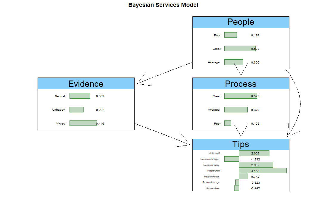
Finally, let’s plot out our new model with node information.
## Updated Model Chart
graphviz.chart(bn.mod,
type = "barprob", bar.col = "darkgreen",
strip.bg = "lightskyblue", main="Bayesian Services Model", bg="white", scale = c(3,5))
From the People-Great coefficient in Tips which we use to proxy customer satisfaction, we can see that people have the greatest impact on customer experience. This confirms that people are our strength which is a touching note to end the article on.
Conclusion
Bayesian networks are a helpful way to reason about conditional probability, assess risks, and run scenarios. They combine human expertise with known data which leads to better decision making when dealing with uncertain outcomes that depend on uncertain factors. They are also a lot of fun!
Recent Post
DAX Calculated Columns with EARLIER
- 20 July 2024
- 5 min read
Exploring Tidymodels Machine Learning Framework
- 17 July 2024
- 7 min read
Bayesian Binomial Product Analysis
- 14 July 2024
- 6 min read
Product Analytics with Binomial Regression
- 13 July 2024
- 12 min read
Flexible Bayesian Modeling in Stan
- 8 July 2024
- 13 min read


