With advances in computing power Bayesian statistics are becoming more popular. Rather than find a representative sample to explain a population, we instead determine the most likely generating process given our data, and then use that process to simulate possibilities.
The advantages of this approach are that it makes it much easier to answer questions and run scenarios. The process also lends itself well to producing a credible distribution of outcomes from which we can set our expectations.
Let’s explore how we can use Bayesian linear modeling to identify a range of predicted volume given various price points.
Results
We determine that the expected profit given $1,500 in fixed promotion cost and a margin of $2.50 is $6,400.
Follow along in R studio to see how we arrived at this result.
Data Generation
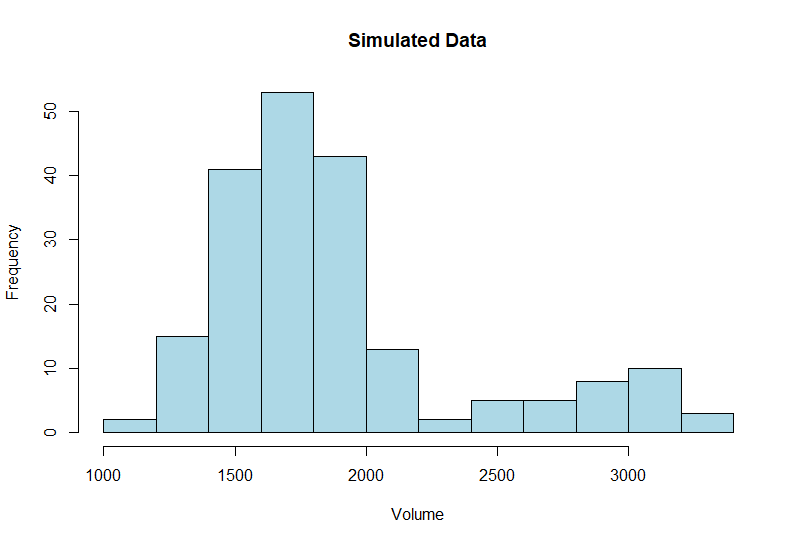
We start with generating some linear sales data for on-sale and regular price periods. We will generate 150 sample observation which is tiny, but this will help demonstrate the effectiveness of Bayesian analysis even when observed data is scarce.
First we will graph out our simulated data. We have a typical bi-modal sales distribution with a second peak during promotional periods.
hist(Simulation$Volume, main = "Simulated Data",
     xlab = "Volume",
     col = "lightblue")
Scale Variables
We will scale our variables since volume is much larger than price. Once that is completed we will run an ordinary linear model in R to get a reality check and an idea of where to set our stan_lm prior for the coefficient of determination (R-Squared).
### SCALE THE DATA
Sim.Scaled <- mutate(Simulation, Price = scale(Price), Volume = scale(Volume))

#### Frequentist Linear Model
lm <- lm(Volume ~ Price + SaleFlag, Sim.Scaled)
summary(lm)
Call:
lm(formula = Volume ~ Price + SaleFlag, data = Sim.Scaled)

Residuals:
     Min       1Q   Median       3Q      Max
-1.08179 -0.31492  0.02272  0.31475  1.45237

Coefficients:
             Estimate Std. Error t value             Pr(>|t|)
(Intercept)  -0.32147    0.03810  -8.438  0.00000000000000687 ***
Price        -0.17945    0.04638  -3.869             0.000149 ***
SaleFlagSale  2.07397    0.12784  16.223 < 0.0000000000000002 ***
---
Signif. codes:  0 ‘***’ 0.001 ‘**’ 0.01 ‘*’ 0.05 ‘.’ 0.1 ‘ ’ 1

Residual standard error: 0.4601 on 197 degrees of freedom
Multiple R-squared:  0.7904,	Adjusted R-squared:  0.7883
F-statistic: 371.4 on 2 and 197 DF,  p-value: < 0.00000000000000022
The R^2 is around 0.8 which could make a decent starting value for the prior information if we run a stan_lm function.
Scaling Factors
Next we’ll collect the center and scale values so we can re-adjust our coefficients and predictions back to the original scale. To center and scale we subtract the sample mean from each data point and divide by its standard deviation. We will have to undo those steps later.
Next we can run our linear model using the stan_glm() function from the package rstanarm.
Specifying family = “gaussian” for a generalized linear model (GLM) will run a linear model without the restriction of specifying a prior distribution for the R^2 which are imposed by the stan_lm() function.
For our summary, we will specify percentile breaks in 10% intervals to get a more detailed picture than the default settings.
stan.glm <- stan_glm(Volume ~ Price + SaleFlag, family = "gaussian",
data = Sim.Scaled)
summary(stan.glm,probs = seq(0.1, 0.9, by = .1))
Basic Diagnostics
Part of the model output will give us Rhat values. Any values above 1.0 indicate problems with model convergence. This is a helpful check although other problems can still be present even if Rhat is 1.0.
In this context a lack of convergence indicates that the sample space is not being explored appropriately and estimates will be unreliable.
The second parameter n_eff refers to the “effective sample size” which is the number of samples during simulation.
Our basic diagnostics look fine so we can continue.
Estimates for our price coefficient range from -0.2 to -0.1. The narrow band indicates certainty of the estimates.
A great feature of the Bayesian approach is that we don’t have to be concerned with p-values and statistical significance, we are instead interested in the credible range of the data generating process given the available data and, where appropriate, our prior understanding.
Coefficients / R2
Everyone loves R^2 values but Bayesian methods don’t have them and trying to find them to some extent misses the point of using simulations. To get around this we will run a Bayesian version that simulates R^2 just in case someone more used to frequentist methods asks about it.
The average coefficients are nearly identical to the ordinary linear regression above, as is the simulated version of R^2.
Bayesian Analysis
You may be asking, given similar results, why would we want to bother with the process of simulating samples. There are two reasons, the first is that there is a lot more flexibility in modeling complex probability with Bayesian approaches.
The second reason is that even though this is a simple linear regression, the output from our Bayesian approach is a lot more useful.
Extracting Chains
Below we will extract the estimations for our coefficients and then use them for our analysis. These chains are our sampled parameter estimates (thetas).
Chains <- as.matrix(stan.glm, pars = c("(Intercept)", "Price", "SaleFlagSale"))
head(Chains)
For example, the coefficient value for SaleFlag bounces around a random normal distribution learned from the data. It is not the same each time, so over a lot of iterations we can get an idea of likely combinations of values.
Plotting Simulated Values
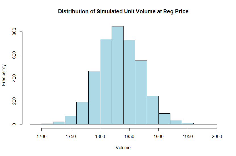
We will plot out a histogram using these chains to better understand what volumes we can expect for a regular price of $6.50 which is equivalent to approximately -0.3 with our current scaling.
To get sensible results from the chain we need to input our scaled price and indicator flag into the formula: Volume = PriceCoef * -0.3 [Price] + OnSale * 0 [NoSale]. Then we have to unscale our prediction by multiplying it with the standard deviation for volume and adding back the mean.
hist((Chains[,1] + Chains [,2] * -0.3 + Chains[,3] * 0) * sd.vol + xbar.vol,
     main = "Distribution of Simulated Unit Volume at Reg Price",
     xlab = "Volume",
     col = "lightblue")
We can expect that with a price of $6.50 our volume will be around 1,825 but occasionally it might be as low as 1,700 or as high as 2,000 with various levels of likelihood roughly following a normal distribution.
ProbabilityScenario
We can also use our chains to determine the likelihood of seeing 1,900 units given a price of $6.50 by relying on the mean() function in Base R. The mean function can be used to count the number of times an expression is true out of all executions, due to true/false being treated as 1/0 this ends up being the probability of an outcome.
The probability of hitting 1,900 units is 3.5% given a price of $6.50.
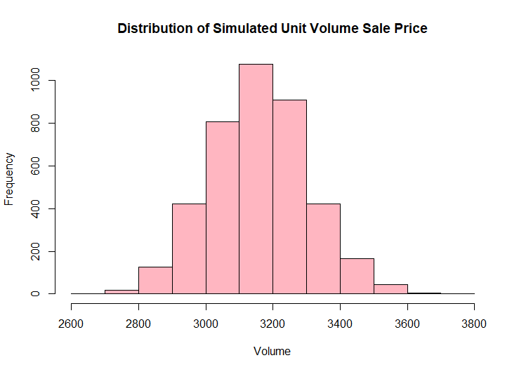
Now let’s take a look at the possible outcomes given that the item is promoted.
hist(((Chains[,1] + Chains [,2] * -0.3 + Chains[,3] * 1) * sd.vol + xbar.vol),
     main = "Distribution of Simulated Unit Volume Sale Price",
     xlab = "Volume",
     col = "lightpink")

mean(((Chains[,1] + Chains [,2] * -0.3 +
Chains[,3] * 1) * sd.vol + xbar.vol) > 1900)
The same item promoted at $6.50 has a 100% probability of seeing at least 1,900 units sold. A much rosier picture to be sure.
The great thing about Bayesian analysis is that we can easily modify this scenario to find out what our expected value would be given that our margin is $2.50 and the cost of promotion is fixed at $1,500.
The expected value of this new scenario is that we would make ~$6,400 in gross margin after the cost of the promotion. We could just as easily explore the distribution of margin outcomes or the probability of margin exceeding some value.
There is huge benefit of using the Bayesian approach for business problems involving risk and uncertainty. This approach makes it easy to compare the above result against not running the promotion, or even to find the maximum value we would be willing to pay for the promotion given our risk tolerance.
Stan Linear Model
Next let’s fit the same linear model, but using the stan_lm() function instead. We will also load shinystan which builds a “Shiny App” for easy viewing of model diagnostics and results.
For this function we have to specify a prior distribution for R2 which is based on a beta function, a popular choice for modeling probabilities. This is an informative prior that helps fit the model coefficients, we will specify 0.78 which is what we arrived at using frequentest calculations for R2.
As it happens the default prior is based on the mode of the beta distribution which requires more than two parameters. Since we only have two we will instead use the median.
We will also specify a smaller value of adapt_delta which has the effect of reducing the “step size” of the sampler. The default is 0.95, so we will crank it up to 0.999 to avoid too many divergent transitions (They are coming!).
We experienced 8 divergent transitions which suggests that we should probably review and possibly re-parameterize the model. These often arise because the sampling algorithm gets stuck in very narrow areas and they can sometimes be fixed by lowering adapt_delta.
Lowering this parameter will always improve the sampling and decrease the size of the steps the algorithm takes, but at a cost of extra processing time which could render the problem intractable for a larger model.
In this case it seems to result from having to use this type of prior on a two parameter model since we did not have the issue with the glm version that defaults to a non-informative prior.
In any case, just for fun let’s see how this model stacks up to the glm version.
Our coefficients are nearly identical suggesting that it is probably usable even with a few divergent transitions. We could also extract the chains and plot the distribution, if we did so we would find that it looks almost the same as the glm version.
We want to avoid divergent transitions if possible, but a small number may not be the end of the world in a business context provided we get convergence.
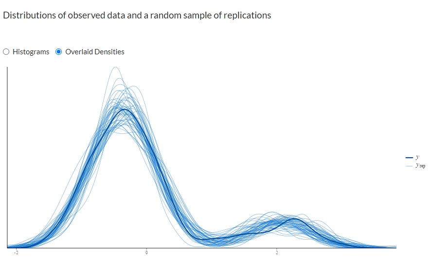
Shiny Stan Diagnostics
In ShinyStan we can select “posterior predictive checks” and look at how our sampled distributions compare to the original. In this case they line up very well for 150 data points.
shinystan::launch_shinystan(stan.lm)
There are a host of other interesting diagnostic tools available that are worth exploring in ShinyStan such as multivariate plots to track down the source of divergent transitions.
We can also get an idea what our distribution looks like (right) for divergent transitions compared to normal (left). This one looks like it’s been stepped on which is not what we want to be sampling from, especially if there are a lot of these issues.
Conclusion
The rstanarm package makes running standard models such as linear or generalized linear models in the Stan probability language almost as simple as running their counterparts in Base R.
While the Bayesian approach does still add a bit of complexity compared to more familiar approaches in statistics the benefits are well worth it. In a business context these approaches allow us to run scenarios and determine likely ranges of outcomes which is helpful in assessing risk and reward.
More on Stan
A slightly more in-depth (but not too technical) look at Bayesian MCMC sampling and the Stan language is available in a follow-up article: Flexible Bayesian Modeling in Stan.