Interpretative machine learning is a powerful tool to understand customer decisions, including willingness to pay for specific features. This is an iterative process that starts with training a model that does well at predicting the thing we are interested in. Once trained we can query our model to gain insight into important factors and run scenarios that can help with development initiatives.
Let’s explore how we can use mlr3 and interpretive machine learning to better understand the contribution of features to vehicle prices.
Using several machine learning models we determine the contribution of various features to sedan price and find evidence that increasing size and horsepower will result in a $10,000 – $15,000 improvement in selling price. Further that we can increase horsepower less to achieve the same effect provided we make the body size more impressive.
Follow along below in R Studio to see how we arrived at this result.
Loading Data
Our first step is loading our required packages, data from CSV, and then wiping out a few variables that will not help with the this particular task.
Given the size of the remaining variables it is a good idea to see if any others can be discarded for lack of predictive information. That will keep our model more parsimonious and potentially help with predictions.
We will use the Boruta package which uses Random Forest variation of feature selection. Unlike maximum relevance minimum redundancy (mRMRe) this algorithm looks for all relevant features. This makes it a great choice for a small data set of vehicles where we might have interactions between different predictors.
We will also be using a random forest model and they tend to handle redundancy quite well so it is less of a concern.
Boruta performed 45 iterations in 0.8729489 secs.
 20 attributes confirmed important: aspiration, boreratio, carbody, carheight, carlength and 15 more;
 1 attributes confirmed unimportant: doornumber;
Boruta is very optimistic on our feature set although some are definitely more relevant than others. The only feature that receives the axe is the number of doors.
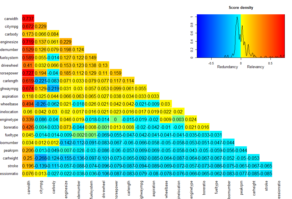
We will also check out the mRMRe method which focuses on features that are highly relevant but not redundant. Unsurprisingly this data contains some fairly redundant features because things like cylinder number would tend to have a lot of correlation with horsepower.
With the varrank package we are interested in the numbers on the diagonal. They are ordered from most to least relevant.
Very well. Both agree that door number is not relevant for our vehicle prices. If we need to chop off some more variables we can revisit this chart, but for now we will stick with everything that is relevant and only remove door number.
CreateTask
The MLR3 package is a great framework for R that allows us to create a modular analysis setup. At first it seems a bit cumbersome, but when we want to run a number of different experiments a little bit of work on the front end can save a huge amount of time.
The first one these modules is a task. In this case we need to create a regression task because we are interested in predicting numeric car prices.
The next module we need to create is a learner. We will actually create three of them and let them duke it out to see which one will have the privilege of being our chosen model. Only the chosen model will be blessed with seeing our holdout data before we run real analysis.
We will create:
An Elastic Net model which is a penalized version of linear regression.
A Random Forest model which is a collection of randomized decision trees that will confer together and vote on car price as a group.
An XGBoost model which is a more intelligent (but also more complex) version of a random forest.
While we create them we will also specify some tuning parameters. MLR3 uses a package called paradox to manage tuning so we will specify those with P_datatype() within the to_tune() function of the learner definition.
Now that we have three learners we need to consider whether they are compatible with our data features. Machine learning algorithms commonly have a hard time with categorical data.
Random Forest is extremely flexible so we can mostly run it as is. However, XGBoost and Elastic Net will require feature encoding. Thankfully this is a breeze with MLR3 pipe operators.
Pipe Operators
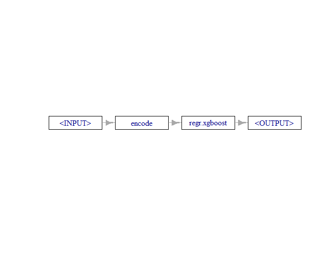
There is more information on Pipeline Operators in this article so we won’t dwell on it here except to say we are creating a flow chart (or DAG if you prefer) from encoding to learner, and then taking that entire process and telling MLR3 to treat it as a learner. When we train our model these pipelines will be the learner we reference for both XGBoost and Elastic Net.
Next we will set up some options for parameter learning specifying five fold cross validation and a tuning grid resolution of 100. We will look to minimize Root Mean Squared Error (RMSE). If our model has a lower RMSE then it is hitting the mark more often.
The terminator has no relation to the movie, it is the stopping criteria for training. Since we are using an exhaustive grid search we will set it to “none” and grab a coffee.
First we will train our Elastic Net model with four processors working on the task. In MLR3 this is done with a tuning instance that will return the optimal hyper parameters for training.
The tuner will cover the parameter space using five fold cross validation in order to determine the best settings for lambda (called “s” in the tune grid) and alpha. These two parameters determine the character and amount of penalization for our linear regression model.
Grid search takes a long time with five fold cross validation even for a relatively simple model. We trained our model on 1,000 combinations of 2 parameters with 5 rounds of cross validation for each pair.
Now that we have our first tuned model we can clone the learner to make a new copy, note that otherwise MLR3 uses references similar to Python. Next we set the parameters values on our cloned model, and then we train, careful to include only the training partition with the row_ids argument.
The model can be accessed under GPipeTuned$model and we can also test predictions on our unseen validation data and calculate a RMSE score.
Our tuning process has settled on a pure ridge regression model with a fairly high penalization term. The RMSE on the validation date is $3,400 which is alright, but not amazing. To improve this we might try standardize the data, add interaction terms, or transform some of the variables.
We’ll leave it for now and see what kind of performance we get from the other candidates. This time we will try using “mbo” tuning which is a Bayesian optimization algorithm that is likely to much faster than a grid search for XGBoost models. For our terminator we will specify 120 seconds runtime.
The Random Forest model performs better on the validation set with RMSE of $2,124; but we will also run a benchmark between our three models and another learner called “featurless” which just provides a prediction baseline.
MLR3 makes it very easy to benchmark different models, we simply set up an experiment with a list of learners and a resampling strategy and it does the rest.
We can confirm that the Random Forest model has ousted its competition and performs much better than our baseline learner.
Notably, Elastic Net had a respectable score benchmarking but that did not translate into the validation score suggesting it may be overfit or over parameterized, or it may have got a bad shake with validation data. Regardless, it was the worst performer in both tests.
Final Training
Now that we have selected a final model we will train it on all of our data by removing row_id settings and allowing it to train on both the train and test sets. The idea here is that adding extra data will reduce the variability of predictions without causing any additional bias because the parameters are already determined.
#Train the Chosen Model
RFLearnerFinal = RFLearner$clone()
RFLearnerFinal$param_set$values = instance$result_learner_param_vals
RFLearnerFinal$param_set$values

RFLearnerFinal$train(PriceTask)$model
Shapley Analysis
One of the disadvantages of tree models is that they become a lot more difficult to interpret than simple models like linear regression. Although to be fair a regression model with 45 parameters is no picnic either.
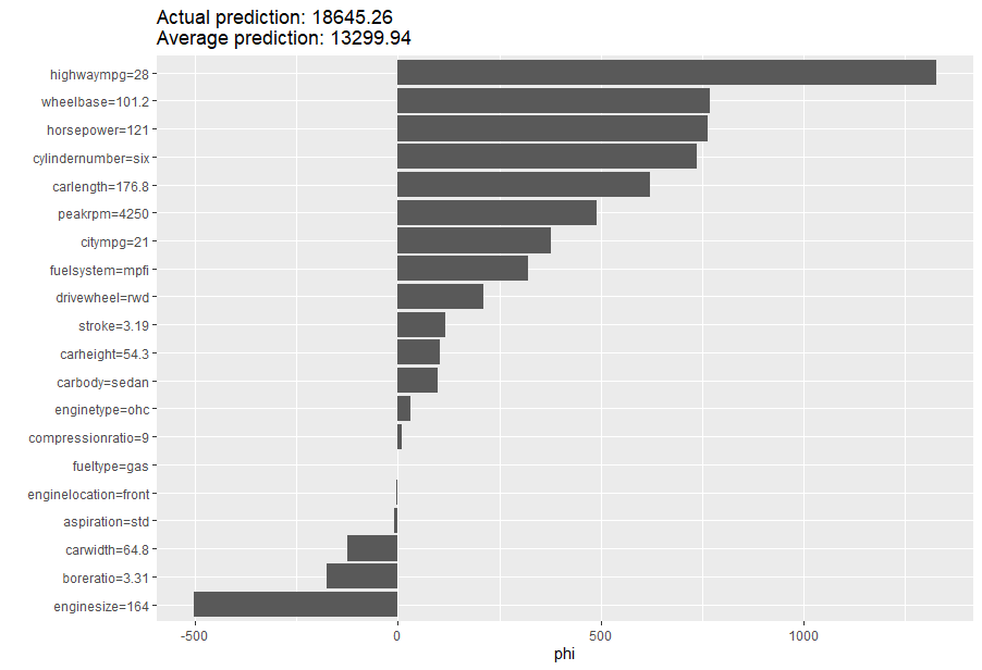
One way to get insights into how models are making decisions is Shapley values. These values estimate the marginal effect of each variable on the prediction. We are going to explore row 14 of the data set which is a six cylinder sedan costing $21,000.
To run the analysis we will use the iml package which stands for interpretable machine learning. This package is part of the MLR3 ecosystem.
The first step is to convert our learner into a Predictor object by passing the model, the original dataset, and specifying y = “price” as the response variable.
CarPrices[14,]

mod <- Predictor$new(RFLearnerFinal, data = CarPrices, y = "price")

shapley = Shapley$new(mod, x.interest = CarPrices[14,],
                      sample.size = 1000)
shapley$plot()
shapley$results
The Random Forest Model placed a lot of emphasis on highwaympg, wheelbase, and horsepower. It did under predict on this example, but only by about the amount of the RMSE score.
We will also check how the Elastic Net regression model compares since it uses a very different approach.
mod.glm <- Predictor$new(GPipeTuned , data = CarPrices, y = "price")
ShapGLM = Shapley$new(mod.glm, x.interest = CarPrices[14,],
                      sample.size = 1000)
ShapGLM$plot()
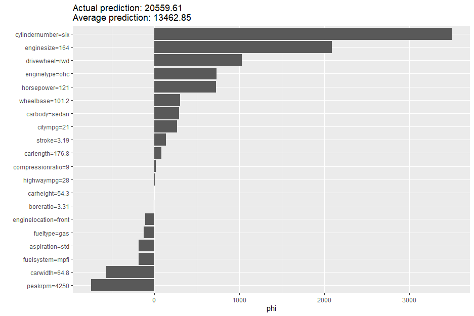
Our elastic net model actually out performed the random forest model on this specific prediction, only undershooting the actual value by $500. Although, in general the random forest model has much better performance.
Some key differences are emphasis placed on engine type and engine size. Perhaps those are more relevant to sedan customers, or perhaps it was a lucky guess. We might want to look at performance for some other sedans and see if there is a pattern.
Counterfactuals
Counterfactual analysis can help ask questions from our data such as: “given that the price of this vehicle is $21,000 what features would cause it to be worth $30,000?”
We can run these analysis with the help of the counterfactuals package using the same type of Predictor object we created above. We will specify 2 counterfactuals, and a range between $30,000 and $35,000 for our sedan.
Of the two scenarios returned both suggest that adding size to the car body and extra horsepower would bring the price up to $30,000. The second option suggests that we can get away with less horsepower if we add a more impressive body size.
Conclusion
Interpretive machine learning helps us leverage human intelligence by providing managers with important insights on customer preferences or buying behaviour. We’ve seen how we can use machine learning tools to identify important features and run counterfactual analysis to improve business outcomes.
MLR3 is a cutting edge machine learning framework for R that makes the entire process a breeze. There is a free ebook available at the link below where you can learn more about the platform.