One of the most common questions in retailers want to know is what their customer’s basket contains. A more savvy extension of this is to consider the role each product plays in the retail space.
Network graph models can help us understand the importance of products, relationships between them, and their relationship to our customers.
Let’s explore using frequent item sets and graph functions to better understand our product offering.
Results Overview
We find that our most important product is milk, and one of our least important products is spices. We also determined that bottled beer, pip fruit, and bread rolls are close neighbours of canned vegetables.
Follow along below in R Studio to see how we arrived at this result.
Dataset
For this example we will be using the very popular Groceries dataset available on Kaggle. This dataset contains three columns for membership number, transaction date, and item description.
This is a great dataset both because it focuses on the customer identifier rather than the transaction code, and also because it has a categorization system that strikes a good balances between specific and general.
Load Data
First we will load our required packages. The arules package will help us find common item sets, and the igraph package will provide support for graph functions and vizualization.
We will also do some light cleanup since no-one loves excessively long variable names.
Our goal is to represent various products as nodes in a graph model. The edges that connect these nodes will be the customers who purchase both of the items. The the strength of a relationship will be based on the number of customers who purchase both items.
Frequent Itemset
The first step is to build a transaction object based on the MemberID and ItemLabel. Typically we would build this on the transaction number, but in this case we are interested in what customers are buying over time, not what is in a bag walking out of the shop.
Building transactions on the customer identifier is like understanding what the customer keeps in their fridge, rather than what they happened to be out of some Friday when they dashed in to pick up a few items.
Trans <- transactions(Groceries, format="long", cols=(c("MemberID", "ItemLabel")))
Apriori Algorithm
Apriori is an efficient algorithm for creating frequent itemsets, it uses a bottom-up approach in searching for candidates. Without this type of heuristic the number combinations to consider would quickly become intractable.
We are interested in graphing the relationships between nodes representing products. Those nodes will be connected by edges that represent a customer who purchased both items. More on this later, but to obtain sensible results we will need to have rules with a length of exactly two.
The other parameter is support, we might consider this the popularity of the product. This is a cutoff representing the basic probability of the item being purchased by a customer. That is the number of customers who bought the item divided by the number of customers.
Setting support is normally a bit of trial and error. If the number of rules returned is too large to be useful we can increase the support requirement, if the number of rules are too few then we can decrease the support.
Our algorithm reports that it has discovered 2,099 frequent itemsets of length 2, and the minimum level of support is a product purchased by 19 customers.
Creating Edges
To create our edges list, that is the connections between our products, we will need to put the frequent itemset into a dataframe and do a bit of cleanup.
Apriori results are stored in a S4 object. We can extract item support for the edge sizes with the ‘@’ operator. We can also retrieve the labels with the labels() function.
freq.df <- data.frame(
  itemset = labels(freq.items),
  support = freq.items@quality)

head(freq.df)
This provides us with absolute support numbers, and the itemsets in a character format. Unfortunately, the itemset column is surrounded with curly braces so we need to clean this up prior to analysis.
Cleaning Itemset
The first step in cleaning the output is to remove the curly braces “{}” with str_replace() from the tidyverse stringer package. We have to use “\\” to double escape the regex.
Next we break out the comma separated items into their own columns with seperate().
With a clean dataframe we can now create an edge list. Each edge has a start node and destination node, and the strength of the relationship is determined by the weight. In this case, weight represents the number of unique customers who have bought both items over some period of time.
To get a sense of the connections in our data we can look at the summary of edge weights. If we would like to focus on more important relationships we can cull some of nodes and edges that have lower weights.
> summary(edge.list$weight)
   Min. 1st Qu.  Median    Mean 3rd Qu.    Max.
  20.00   27.00   41.00   64.64   74.00  746.00
Creating a Graph Model
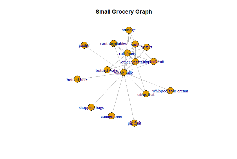
Let’s visualize a small subset of our product graph to make things a bit more concrete. We can do this by creating a graph from the edge list dataframe.
Since frequent itemsets are not directional we will also convert our graph to undirected using as.undirected() which defaults to creating one edge per pair of nodes with any directed edge.
Somewhat ironically, large graphs are impossible to decipher so it’s often easier to either use calculated measures or visualize a smaller slice.
We will leave all our edges in for now and create an igraph model with all of our nodes.
g <- graph_from_data_frame(network.data)
With our model we can now start running some preliminary analysis. Graph models have a some very useful measures of importance.
Centrality Measures
A favourite is Eigen Centrality, this measure is often described as a “prestige” score for a node. That is how many connections are there to the node, and how many of those connections come from other important nodes.
This is similar to a popular professor in college who is always surrounded by popular leaders from other faculties. We would say that person has a good deal of prestige.
We can see that our most prestigeous items are milk, veggies, rolls, and soda. Our least prestigeous items are dental care, spices, brandy, sauces, and meat spreads.
This gives some credence to the idea that milk should always be at the back of the store because it forces customers to walk through the aisles.
In any case, centrality measures are a very efficient way to rank each item in our store by its relative importance to our customers. This could be useful in controlling price perception by ensuring pricing is competitive on items important to our customers. It could also assist with placement, perhaps dental care impulse buys should be next to the soda.
In addition to Eigen centrality there are other scores such as betweenness, and the Kleinberg hub score. In practice, they tend to identify similar items.
EdgeDegree
Degree is another property of graphs. The degree is simply the number of connecting edges each node has. In the retail context that would mean the number of other items that are bought with the target item.
As it happens, the items with the highest degree are more likely to be connected to other important nodes, and also have a high centrality score due to the number of connections. Again, results are similar but it’s a different way of looking at importance.
degree(g)[degree(g) > 90]
> degree(g)[degree(g) > 90]
            soda       rolls/buns other vegetables  root vegetables           yogurt       whole milk
             104              109              106               92              100              116
Good Neighbours
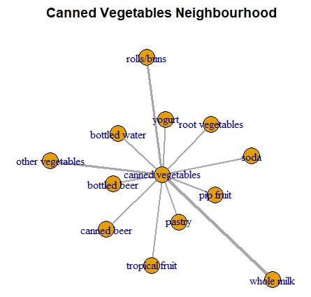
Another way to explore our products is to look in the neighbourhood and see what other items have purchase support with an item of interest.
We can use the neighbourhood() function to find other nodes near our target node and then create a smaller sub-graph to analyze.
Although it may be interesting to look at connections between other items in the neighbourhood in addition to those they have with our target, we can also remove them by identifying the set difference of incident edges.
Finally, we will set the edge width to more easily see the neighbours with the strongest connections and plot the result.
The neighbourhood of canned vegetables includes other vegetables, bottled beer, and pip fruit.
CustomerConnection
Once we have a graph set up it is often useful to in conjunction with techniques such as clustering. Rather than look at all of our customers, we may be more interested in which products resonate the most for a specific segment we are attempting to target.
To do this we simply remove the customers we are not interested in from our original transaction list and re-run the above analysis.
The possibilities are almost unlimited for graph exploration, this article only touches the very tip of the proverbial iceberg.
Once we have identified our products and linked them together we can perform incredibly insightful analysis, and repeat it quickly for customer segments or particular locations.
References
Luke, D. A User’s Guide to Network Analysis in R. Springer (2015).
Kolaczyk, E.; Csardi, G. Statistical Analysis of Network Data with R. Springer (2020).