A fundamental law of economics is the relationship between price and volume. Pricing is the key mechanism through which markets efficiently mediate supply and demand. Retailers that do not have efficient pricing, especially in a challenging economic situation will leave margin dollars on the table.
A key benefit of price optimization over a strategy such as surfing competitor flyers is that it brings our unique cost structure and customer base into the decision making process.
Let’s explore how we can use multiple linear regression models to identify price volume relationships and use them to optimize our price and maximize margin to costs.
Data Required
For this example we will confine ourselves to average weekly sales price, weekly unit volume, and an indicator for whether the product was on sale. We will look at a 100 week period, or roughly two years of data.
Results
Optimizing Product A’s price based on its estimated demand curve and a unit cost of $5.99 we find that the optimal regular price is $12.24 resulting in an expected weekly margin of $4,444. To see how we arrived at this result follow along with the example below.
Category Optimization
In part two of this post we will explore maximizing margin across a category of products.
SimulatedData
Naturally we need some data. Let’s simulate sales data by using a function that assigns some price variability to a baseline level and adds a proportion of sales lift in weeks the products are on-sale. We will call these products A,B, and C.
library(tidyverse)

## Simulate Data
GenSales <- function(X = 1, Multi = 200, Base = 50, Mean = 100, SD = 50, StartPrice = 2.99) {

    OnSale <- rbinom(X, 1, prob = 0.1)
    Price <- seq(1,X, by=0.01)[1:X] * StartPrice
    Price <- Price - OnSale * Price * sample(c(.1,.15,.20), X, replace = T)
    Units <- round(Base + (Price * -1 * rnorm(X, mean = Mean, sd = SD)) + OnSale * rbeta(X, 2, 2) * Multi, 0)
    Units <- ifelse(Units < 0, 0, Units)
    return(data.frame(Units = Units, Price = Price, OnSale = OnSale))
}
set.seed(56)
PA <- GenSales(X = 100, Multi = 500, Base = 2000, Mean = 100, SD = 25, StartPrice = 5.99)
PB <- GenSales(X = 100, Multi = 5, Base = 150, Mean = 3, SD = 1, StartPrice = 10.99)
PC <- GenSales(X = 100, Multi = 250, Base = 1000, Mean = 20, SD = 5, StartPrice = 6.99)
Multiple Linear Regression
Linear Regression is where we plot out different price points and their unit volumes on a two dimensional scatter chart and try find a line that fits the pattern. The best fitting line minimizes the sum of squared errors (called residuals).
This is a convenient way to get a continuous estimate of what the expected value of unit volume would be at various price points even if we haven’t used them the past.
R makes running MLS a breeze, let’s use the lm() function with the formula: Unit Volume explained by Price and OnSale indicator. (Units ~ Price + OnSale).
Call:
lm(formula = Units ~ Price + OnSale, data = PA)

Residuals:
    Min      1Q  Median      3Q     Max
-480.12 -161.31   13.67  153.20  541.24

Coefficients:
            Estimate Std. Error t value             Pr(>|t|)
(Intercept)  2102.22     110.67  18.996 < 0.0000000000000002 ***
Price        -113.65      12.14  -9.359  0.00000000000000325 ***
OnSale        210.78      88.57   2.380               0.0193 *
---
Signif. codes:  0 ‘***’ 0.001 ‘**’ 0.01 ‘*’ 0.05 ‘.’ 0.1 ‘ ’ 1

Residual standard error: 207.3 on 97 degrees of freedom
Multiple R-squared:  0.5169,	Adjusted R-squared:  0.5069
F-statistic: 51.89 on 2 and 97 DF,  p-value: 0.0000000000000004739
These results tell us that Price + OnSale explain about 50% of the variation (R-Squared = 0.5), that the model is statistically significant (p-value < 0.05), and that each variable is also significant (asterisks).
Product A loses on average 113 units per $1 of price increase, and tends to gain about 200 when it is put on sale independent of the price effect. For the purpose of this discussion we will ignore interactions between price and sales tag.
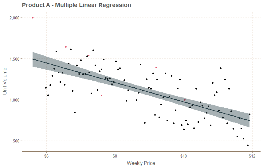
Let’s see what this looks like graphically by running a two variable plot, and colouring OnSale status differently.
ggplot(PA, aes(Price, Units)) + geom_point(col=PA$OnSale+1) + geom_smooth(method = "lm") +
  labs(
    title = "Product A - Multiple Linear Regression",
    x = "Weekly Price",
    y = "Unit Volume"
  ) + theme(legend.position = "none") +
  scale_x_continuous(labels = scales::label_currency()) +
  scale_y_continuous(labels = scales::comma_format())
Our line fits very well minus one outlier near 2,000 units in the upper left. The color indicates it was on sale that week. Handling outliers and influential observations may be the subject of a later post, but visual inspection suggests it is not skewing our model so we will leave it be.
Diagnostics
There are some assumptions we have to meet in order to get the best results from linear models one of those is that the distances of the points away from the line can’t show an obvious pattern, and another is that our data should have a bell shaped (normal) distribution.
Let’s double check to make sure our model is up to code.
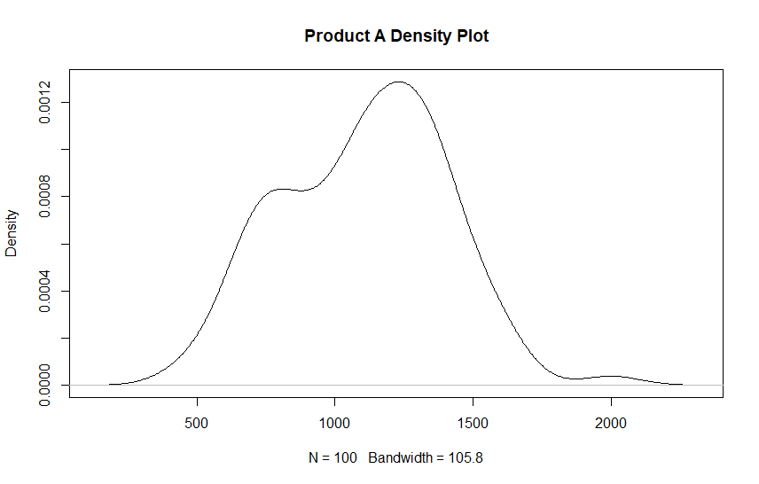
plot(density(PA$Units), main = "Product A Density Plot")
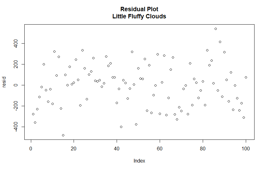
resid <- resid(ols.mod)
plot(resid, main = "Residual Plot\nLittle Fluffy Clouds")
The density plot looks passable, it is not exactly bell shaped but it is fairly typical to see two peaks when dealing with promotional periods so this is not a concern.
The more important assumption is lack of a pattern in the so-called errors which are the distances of the points from the line. The plot above (residual plot) should look like a fluffy cloud. This one may have a very slight pattern but generally points are randomly scattered about zero indicating that it checks out.
Single Product Optimization
Having identified a working model, we now need to define a function that will tell us what the predicted gross margin is given the relationship between price and volume for both cost and sales. Since we are not concerned with maximizing the sale price we leave that coefficient out and assume it is set to zero.
We will use an optimization algorithm from the stats package called optim to find the price point that maximizes our margin.
$par
[1] 12.24328

$value
[1] -4444.302

$counts
function gradient
      NA       NA

$convergence
[1] 0

$message
NULL

> MarginMax(df.opt, 12.24) * -1
[1] 4444.301
Our margin is maximized for Product A at $12.24, and the expected value is $4,444.30 per week. This means if we keep our price around this value it will lead to long-term profits being maximized due to the law of large numbers, even if we miss the mark slightly on any given week.
The most recent price for Product A is $11.90 suggesting we are leaving money on the table and selling ourselves short.
Manual Calculations
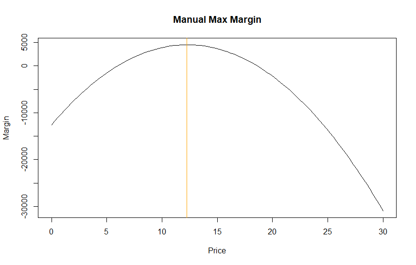
We can check the optimization manually by graphing (Intercept + Slope * Price) * (Price – Cost) = Volume * Margin. Using some basic algebra and substituting known terms from the coefficients we end up with roughly 2779 * Price – 12590 – 113Price^2, a quadratic function that has a global maximum.
### Manual Solution
### (2102X - 113X)(X - C)
MarginManual <- function(x) (2779 * x - 12590 - 113 * x^2)
MarginManual(12.24)
curve(MarginManual, 0, 30, main = "Manual Max Margin", xlab = "Price", ylab = "Margin")
abline(v = 12.24, col="orange")
> MarginManual(12.24)
[1] 4495.571
We can see that using rounded coefficients we get very close to the correct answer with an optimal price around $12.24.
Conclusion
Price optimization is very important for items that have a strong price-volume relationship. Setting price near the optimal level means that over the long term we can expect to maximize weekly our margin.
In part two of this article we explore how to maximize an entire category of products so they work together in harmony.