VARS Product Forecast

Business Insights

There are times when a lot of things are happening in a retail environment which can make forecasting on all of them a real chore. If we’re fortunate there will be a nice smooth trend we can pick out with a low maintenance model like exponential smoothing (ETS).

However, if we need a low maintenance forecast and the interactions between different things happening like price and promotion are making it difficult then Vector Auto Regressive models (VARs) can help make sense of the situation.

VAR models tie different variables together into a single unified model and we may not even need to use any additional external inputs. This is important because if we have to provide future values it can take time, especially if assumptions change often.

By including causal variables directly in the model we can minimize wasted time there will be fewer values we need to anticipate. As an added bonus, where we have two way interactions say between price and traffic counts, the model will naturally capture that inter-relationship.

Let’s explore using a VAR model to forecast product sales.

Dataset

We will use the same data that we used in this article where we discussed ARIMA models. It is a small time series dataset available on Kaggle at https://www.kaggle.com/datasets/soumyadiptadas/products-sales-timeseries-data.

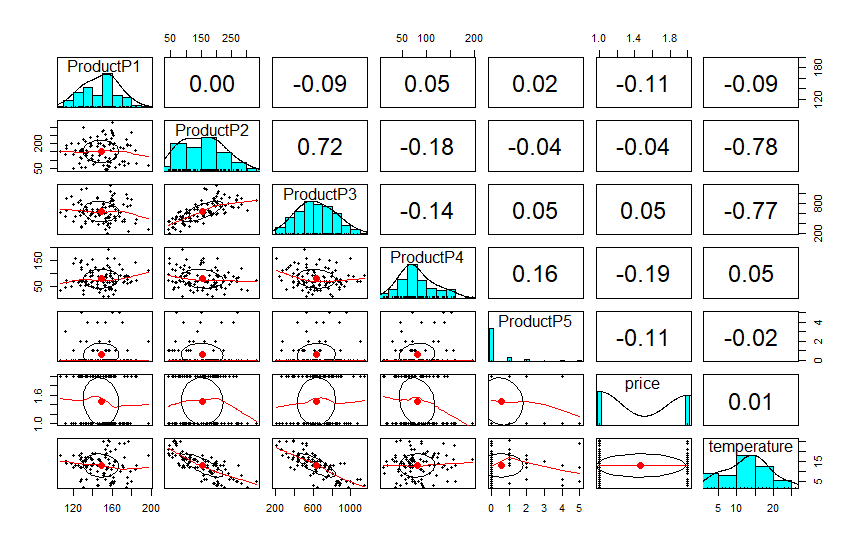
These data are a number of products that have inter-relationships plus price and temperature information. The data are very ill-behaved which makes it a great real world example.

Results

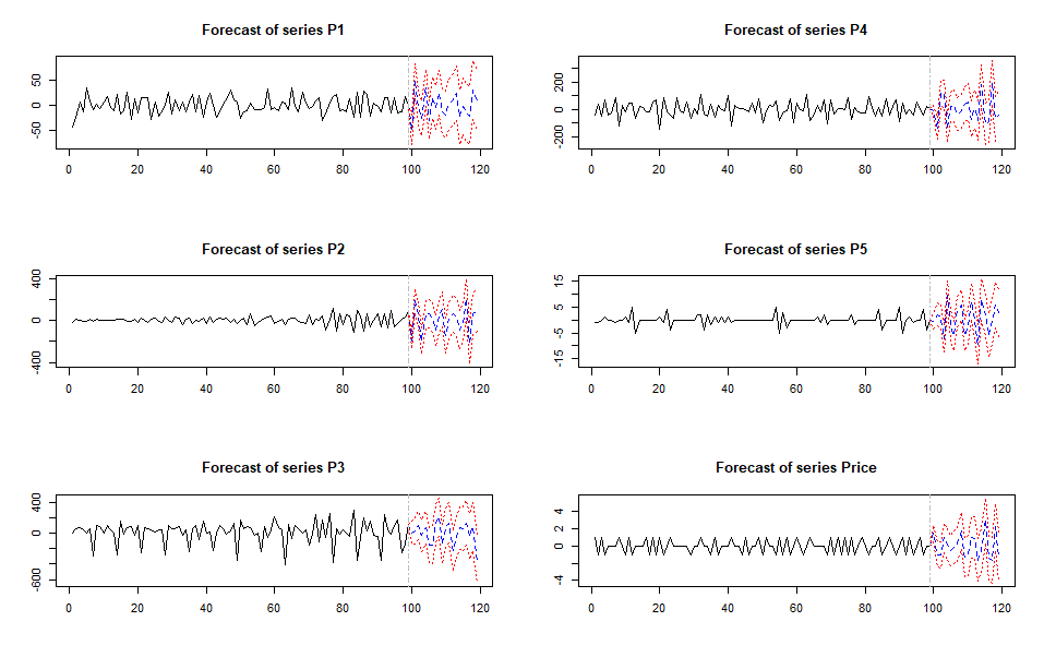
Creating a forecast allows us to make a short term prediction that we will sell 989 pairs of mittens three days from today, with a possible range between 400 and 1,500.

Follow along below in R Studio to see how we arrived at this result.

Exploratory Analysis

Our first step will be to load the 100 series observations and run summary statistics to identify any missing values. There are no missing values so imputation is not required.

Next we will run pairs.panels from the Psych package because it provides a great overview of any correlations within our category of products, plus the price and temperature variables.

library(tidyverse)
library(psych)
library(tseries)
library(MTS)
library(vars)

TimeData <- read.csv("TimeData.csv")
summary(TimeData)
pairs.panels(TimeData[,c(2:7)])

The overview shows us that all but one products have small negative correlation with Price, with P4 being the most responsive.

P2 and P3 have massive correlations with temperature, but the others do not; and what is the most interesting is that certain products have correlations with each other. P4 and P5 have a modest 0.16 positive correlation suggesting they are bought together. P2 and P3 have a massive positive correlation. P3 and P4 have a modest negative correlation suggesting they are partial substitutes.

Given that high temperature will negatively impact the sale of P3 which will then impact the sale of P2 we can see already that this would be fairly irritating to forecast, especially if we had to provide future values for weather and expected sales of related items.

These products could be jackets and mittens compared to running shoes in a clothing store; this type of inter-relationship is very common in retail.

Time Series for P3

We are interested in making an order of P3, let’s call this the mittens and plot the prior sales information.

plot(TimeData$ProductP3, type = "line", main = "Product3 Plot")

What is significant about P3 is that the trend is increasing, possibly temperatures were cooling. There is also a seasonal cycle that occurs about every 7 days, which is not uncommon in retail.

Otherwise, the variations seem irregular. Potentially, this is due to promotional weeks or unusual amounts of snow. It could also be due to promotions on complementary or substitute items .This information may be contained in our other variables.

Creating our Time Series

Feeding several variables into the ts() function in R will return an MTS object, for multi-variate time series analysis.

However, first we will clean up the excessively long variable names. These are not Null Space Approved.  Then we will check all of our variables for stationarity by running an Augmented Dickey-Fuller test and a KPSS test.

Stationarity is a requirement for VARS models to produce good results.

## For those with a distaste for coding long variable names
colnames(TimeData)[2:8] <- c("P1", "P2", "P3", "P4", "P5", "Price", "Temp")
### Check for stationarity
apply(TimeData[,3:8], MARGIN = 2, FUN = adf.test)
apply(TimeData[,3:8], MARGIN = 2, FUN = kpss.test, null="Level")

The ADF test suggests our data is stationary, but these tests are known for false positives so we confirm with a KPSS test. As it turns out both have differing opinions. In this particular case that means we should difference our data where they disagree. Where they agree we will avoid differencing.

For a brief explanation of differencing please see this article on ARIMA forecasting.

KPSS suggests that we should leave Price undifferenced, along with P4 and P5. Following this we will use dplyr to mutate a difference across the other numeric variables.

Finally, we will load our transformed data into a MTS object for analysis.

### Set up MTS Object
Time.mts <- TimeData %>% mutate(across(c(2:4,8), difference)) %>%
  dplyr::select(t, P1, P2, P3, P4, P5, Price, Temp) %>% filter(!is.na(P3))
Time.mts <- ts(Time.mts)

Endogenous Variables

VAR models assume variables are endogenous, that is to say they have a bi-directional effect on each other. For example, high demand causing price to increase, and mittens selling with jackets.

The side inputs are not endogenous, they only impact the model, but are not impacted by the model. In this case we separate out temperature because it is unlikely that sales of mittens affect the weather.

ExoTemp <- as.matrix(Time.mts[,8])
colnames(ExoTemp) <- "Temp"

Above we put our variable into a matrix with column name “Temp” because VAR will complain and rename our variable “exo1” if we simply extract the column from the time series.

Determining Lag Value

Lag values are just the observations that occur after our time series, so today’s lag is tomorrow’s value.

With VAR models we need to specify the number of lags, essentially telling the model how many future periods what happens today will affect. Fortunately, choosing lags is made much simpler with the VARselect function.

We let VARSelect know which variables to use as part of the multivariate structure, those variables will be inter-dependent with each other.

We specify the seasonal period as 7 because there is a weekly cycle; and an exogenous variable for temperature. That is a side input to the model, more frequently called an external regressor.

VARselect(Time.mts[,2:7], exogen = ExoTemp, lag.max = 10, season = 7)
$selection
AIC(n)  HQ(n)  SC(n) FPE(n) 
    10      1      1      4 

Although several options exist for selecting lag, we will generally decide on AIC or AICc. In this case we have no option for AICc so we will use a value of P=10 for our lags. AIC is widely considered the best selector.

Before moving on it is worth mentioning that  for this series VARSelect would choose 13 lags, but this seems like an excessive number. Therefore we cap the number of lags at 10.

If we are unhappy with our results, we can always come back and see how things go with 1, 4, or 13 lags.

Running the Model

Having set everything up to determine our lags, we simply have to use the same parameters and store the model into a variable. The only difference is that we will select P = 10 lags.

Mod.var <- vars::VAR(Time.mts[,2:7], exogen = ExoTemp, p=10, lag.max = 10, season = 7)

Forecast Data

Next we create some data to test our forecast on. We take a recent slice at the end of the time series and then reverse it to simulate a trend reversal in weather. This is converted to a matrix and given the column name “exo1.”

NewData <- rev(Time.mts[80:99,8])
NewData <- as.matrix(NewData)
colnames(NewData) <- "Temp"

Predictions

Next we make predictions with the generic predict() function. We must specify the number of future periods with n.ahead; we will go 20 periods out.

We would now be finished if we had not used temperature as an exogen. Given that we have, we need to ensure that dumvar receives a matrix that is exactly as long as n.ahead.  This is the matrix we created earlier, it contains only values for temperature along with a column name matching our exogen (“Temp”).

pred <- predict(Mod.var, n.ahead = 20, dumvar = NewData)
plot(pred)

Our plots look pretty good, and as bonus we now have forecasts for P3 plus all of the products in our category without having to do any extra work. This is a great feature of VAR models.

Inverting the Difference

Recall that we differened a number of variables, including P3 which is our forecast goal. In order to get useful forecast numbers we will need to undo this differencing operation.

In order to invert a time series with a single difference we have to find the original first observation, and then using that as a starting point and add that to a cummulative sum of the series. i.e. Cumulative Sum(series) + Starting Value.

### Invert Differences [P3]
P3 <- pred$fcst$P3

BeginP3 <- head(TimeData,1)$P3 # Begin of Time Series
par(mfrow = c(1,2))
plot(pred$model$datamat$P3, type = "l", 
     main = "Differenced Data", ylab = "Volume P3")
plot(cumsum(pred$model$datamat$P3)+BeginP3, type = "l", 
     main = "Inverted Difference", ylab="Volume P3")

P3 puffs back up into it’s original glory after this operation. Now we need to apply this to both our pre-forecast and forecast values.

To accomplish this we will first invert the pre-forecast period with the start value BeginP3 above from the head of our series. Next we will identify StartP3 from the tail of the original series.

Finally, we use the apply function with column margin (2) to apply this process to all of the Forecast output. Then work on putting all of this information into a dataframe so it is easier to work with. That will require using NA values to represent points in the pre-period where we have no confidence bounds.

## Pre-Period Cumsum
P3Pre <- cumsum(pred$model$datamat$P3)+BeginP3
## Forecast Start
StartP3 <- tail(TimeData,1)$P3
## Put everything into data frame
P3Fcst <- as.data.frame(apply(P3, MARGIN = 2, FUN = function(x) {cumsum(x) + StartP3}))
P3Fcst
PlotForecast <- data.frame(
  index = seq(1,length(P3Pre) + length(P3Fcst[,1]), by = 1),
  Point = c(P3Pre, P3Fcst[,1]),
  Upper = c(rep(NA, length(P3Pre)), P3Fcst[,3]),
  Lower = c(rep(NA, length(P3Pre)), P3Fcst[,2]),
  Group = factor(c(rep("Pre",length(P3Pre)), rep("Fcst",length(P3Fcst[,1]))))
)

Plotting the Forecast

We can now use ggplot2 to view our forecast for P3. Note that the inverted confidence bounds are omitted to avoid ruining the plot scale.

ggplot(PlotForecast, aes(index, Point, color = Group, group=1)) + geom_line() + 
  labs(title = "VARS Forecast P3 (Inverted Difference)",
       color = "Forecast",
       y = "Product P3 Volume",
       x = "Time Index") + theme_minimal()

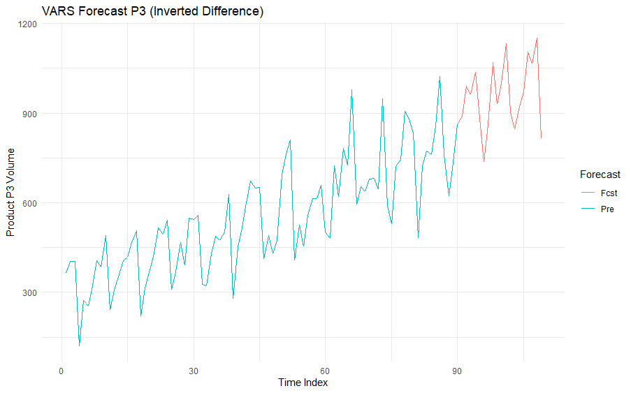
The forecast looks plausible, and from this point we could work on testing and if necessary tightening up some of the parameters.

As it stands, our forecast for three days from now would be 989 pairs of mittens, with a likely range between 400 and 1,500.

Prediction Confidence

The confidence bounds for this model are very large after a few periods, but we could easily run this forecast every day with a new seven day weather outlook.

For an autoregressive model it makes sense that there would be uncertainty for future periods. As we get farther away from the known data because each future observation depends on what comes before it, and eventually on the estimate of the estimate that came before it.

That doesn’t mean that our mitten sales will suddenly hit zero after 100 periods of growth, although that could happen with an early spring. Rather, it reflects the outer bounds model uncertainty due to declining information.

However, provided past patterns hold steady we would expect to see actuals that are reasonably close to the forecasted values and this type of model lends itself well to repeated, low maintenance, rolling forecasts which can be a very useful thing.

Conclusion

VAR models are popular in econometrics because they naturally handle a number of correlated variables that interact with each other. For the same reason they can be very useful in a retail context, particularly for co-dependent products.

They are often not a great choice for longer term forecasts but for short-term forecasts they can be very convenient options because they avoid the problem of having to provide future values. They can be auto-tuned easily, and simultaneously forecast all of the co-dependent variables.

Happy forecasting!

Ax=0

References

Chatfield, Chris; Haipeng, Xing. The Analysis of Time Series: An Introduction with R, 7th Ed. Chapman & Hall/CRC, 2019.

Related Posts

ARIMA Product Sales Forecasting