Customer Clusters with Gaussian Mixed Models

Dustin

22 October 2024
8 min read

Introduction

Clustering customers into similar groups allows us to fine tune marketing strategies such as targeting content based on group membership.

Gaussian Mixture Models (GMMs) are an alternative to commonly used clustering algorithms such as k-means or k-prototypes which we explored in this article.

Class membership for GMMs is determined by customers sharing a common data generating process. This is a different and potentially more precise approach than using distance measures from random starting points.

These models also have some practical advantages, such as being able to provide a probability of cluster membership, and being able to assign new observations to clusters based on those probabilities.

Let’s explore clustering our customers using this method.

Simulate Data

We will simulate some data to get started by created two groups that differ by spending, gender, and income level in thousands. We will represent females as 0 and males as 1.

options(scipen=999)
library(tidyverse)
library(mclust)
library(QuantPsyc)

GroupOne <- data.frame(
Spend = round(rnorm(1000, 500, 50),2),
Sex = sample(c(1, 0), 1000, prob = c(0.3, 0.8), replace = T),
Income = sample(c(500, 600, 700, 800, 900, 1000), 1000, prob = c(0.05, 0.05, 0.2, 0.3, 0.2, 0.2), replace = T)
) %>% mutate(Grouping = 1)

GroupTwo <- data.frame(
  Spend = round(rnorm(1000, 1000, 250),2),
  Sex = sample(c(1, 0), 1000, prob = c(0.8, 0.2), replace = T),
  Income = sample(c(500, 600, 700, 800, 900, 1000), 1000, prob = c(0.3, 0.2, 0.2, 0.1, 0.1, 0.1), replace = T)
) %>% mutate(Grouping = 2)

AllGroups <- union(GroupOne, GroupTwo)

Gaussian Mixture Models

Gaussian Mixture Models work on the premise that there are multiple distributions in the data, and that we can determine class membership based how likely it is that data from say some customer came from a particular distribution.

The simplest case to imagine is a bimodal distribution where we have high spending and low spending customers. Most likely a customer observed spending a small amount will belong to the class of low spending customers.

Expectation Maximization

GMMs are fit using the Expectation Maximization (EM) algorithm which consists of two steps. One step determines the probability of class membership from some starting parameters, and the second step determines the likelihood of parameters given the estimated probabilities of class membership and tries to improve them.

The process repeats estimating class membership and parameters in tandem until convergence criteria are met and we are left with a good estimate of both unknowns.

Taxonomy of GMMs

There are 14 types of cluster models in mclust based the three characteristics of elliptical cluster boundaries (volume, shape, and orientation). A model may have equal volume (size), equal shape, and variable orientation as in the left example. It may also be variable for all three characteristics as in the right example.

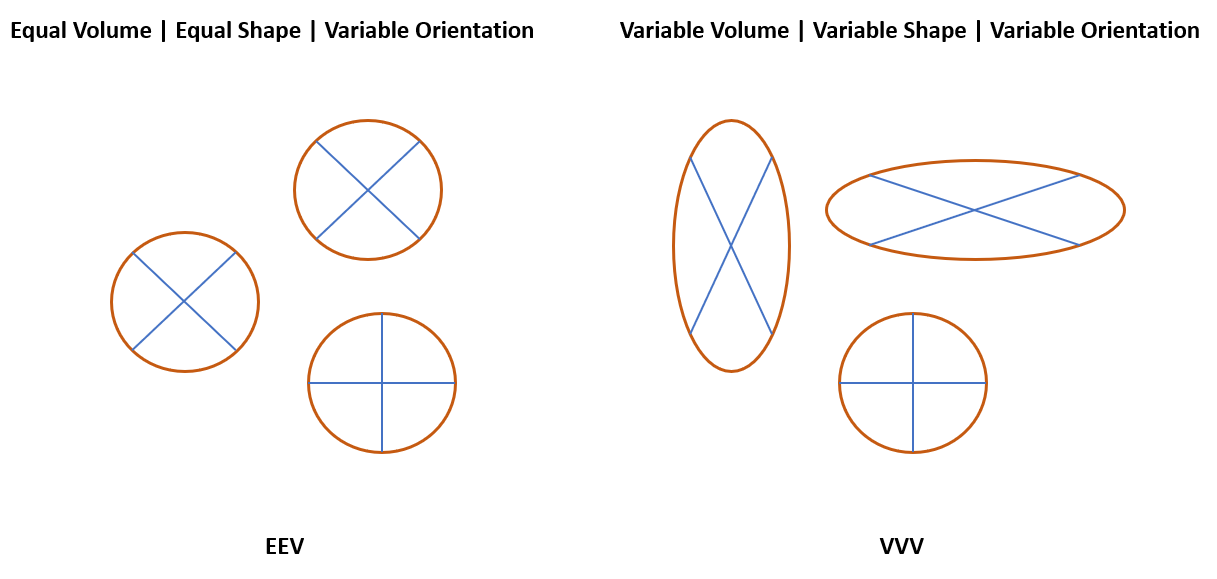
Models are expressed as three letter acronyms where the first letter indicates Volume, the second Shape, and the third Orientation. They can be equal (E), variable (V), or identity (I).

Modeling GMMs in R

The mclust package provides a framework for GMM clustering in R. The function accepts a dataframe and assess up to 16 models with clusters ranging from 1 to 9. Selection of the best model is based on BIC (Bayesian Information Criterion).

Note that some models may end up with NA scores due to singularities appearing in the calculations.

Single Variable Model

We will first explore the simple case with a single variable for spend and run a summary with “Parameters = T” so we can get the full picture of its parameters.

AllGroups.Data <- dplyr::select(AllGroups, Spend)
mod <- Mclust(AllGroups.Data)
summary(mod, parameters = T)

Mclust V (univariate, unequal variance) model with 2 components: 

 log-likelihood    n df       BIC       ICL
      -13382.48 1993  5 -26802.95 -26990.15

Clustering table:
   1    2 
1043  950 

Mixing probabilities:
        1         2 
0.4980619 0.5019381 

Means:
       1        2 
500.5586 983.1254 

Variances:
        1         2 
 2473.606 66706.229

The GMM contains two clusters with roughly equal mixing probabilities. The best model is a single variable model with unequal variances.

We have also mostly recovered the means and variances from our generated data. Cluster One is the first group with a mean spending of $500, and Standard Deviation of $50.

Plotting BIC Scores

We can plot out the BIC scores that were tested and see that the variable model tends to have the best BIC, and the highest point occurs for a two cluster model.

plot(mod, what = "BIC")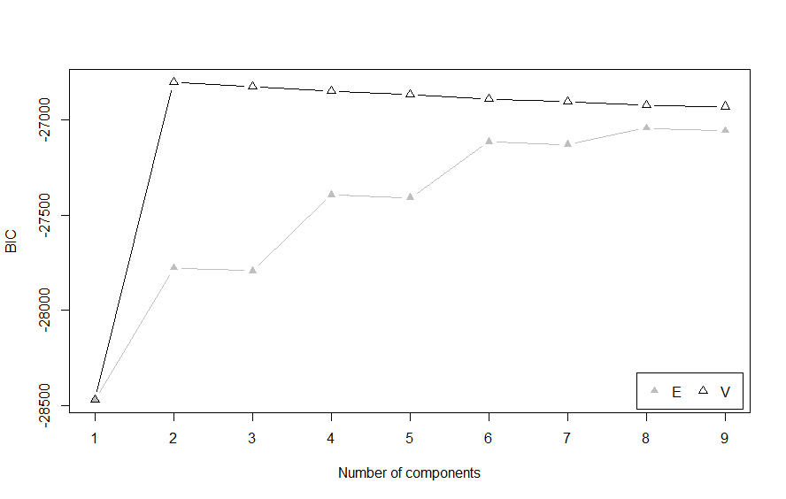

We can validate our clustering against the original classes using the adjusted Rand index (ARI) which is a score between 0 and 1 used to evaluate a clustering solution. The ARI is high at 0.83 and we can see that most of the assignments were made correctly but some overlap remains.

table(AllGroups$Grouping, mod$classification)
adjustedRandIndex(AllGroups$Grouping, mod$classification)

> table(AllGroups$Grouping, mod$classification)
   
      1   2
  1 975  20
  2  68 930
> adjustedRandIndex(AllGroups$Grouping, mod$classification)
[1] 0.8310957

Multivariate Case

We have successfully separated our clusters based on spending. Next let’s analyze our clusters with the other two variables for sex and income level by selecting all variables except the original class assignments.

Since we are using Gaussian Mixture Models it makes sense to verify that we have a normal distribution, otherwise we might obtain some strange clustering results. We will use the “mult.norm” function from the QuantPsyc package to test for multi-variate normalcy.

AllGroups.Data <- dplyr::select(AllGroups, -Grouping)
mult.norm(AllGroups.Data)$mult.test

           Beta-hat      kappa p-val
Skewness  0.9064549 301.547336     0
Kurtosis 12.6035101  -9.773841     0

Testing for Normalcy

The “mult.norm” function runs Mardia’s test. If the p-value is below 0.05 we have evidence to reject the null hypothesis and conclude that the distribution is not multi-variate normal. This is unfortunately the case here.

Unsurprisingly, sex and income do not follow a normal distribution. In the real world it is also quite likely that spending will not be normally distributed.

mod <- Mclust(AllGroups.Data)
summary(mod)
summary(mod$BIC, k = 2)

Mclust VEI (diagonal, equal shape) model with 5 components: 

 log-likelihood    n df       BIC       ICL
      -25736.43 1996 26 -51670.44 -51893.97

Clustering table:
  1   2   3   4   5 
227 283 952 402 132

We might try some transformations in order to force the data into a normal distribution but mclust provides a solution for combining smaller clusters.

Entropy Clustering

In order to avoid a situation with too many clusters created when data is not exactly normal, mclust provides a function called “ClustCombi” to merge clusters hierarchically based on entropy scores. There is a parameter available to specify the model, we will specify “VEI” as that was the best model by BIC score.

Clusters <- clustCombi(mod, ModelNames = "VEI")
plot(Clusters, what = "tree")

Mclust model name: VEI 
Number of components: 5 

Combining steps:

  Step | Classes combined at this step | Class labels after this step
-------|-------------------------------|-----------------------------
   0   |              ---              | 1 2 3 4 5 
   1   |             3 & 4             | 1 2 3 5 
   2   |             3 & 5             | 1 2 3 
   3   |             1 & 3             | 1 2 
   4   |             1 & 2             | 1

In the above summary we can see clusters 3 & 4 were combined, followed by 3 & 5, and so on. This is also represented graphically in the entropy tree.

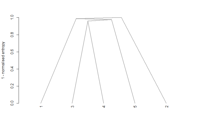
Another option is to look at an entropy plot which takes output from the original model with respect to class membership (z) and the combining matrices from the clustCombi output.

In the example below entropy increases rapidly at four clusters suggesting a four cluster solution, although we know that is not technically faithful to our original groups.

entPlot(mod$z, Clusters$combiM, reg = c(2:6))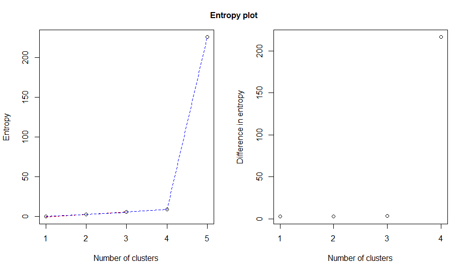

We will optimize the number of clusters by passing the clustCombi result to clustCombiOptim which selects a four cluster solution for us.

We then bind the results with the original classifications and clusters for validation.

Clusters.opt <- clustCombiOptim(Clusters)

FinalResult <- cbind(AllGroups.Data, Cluster = Clusters.opt$cluster.combi, Grouping = AllGroups$Grouping)

table(FinalResult$Grouping, FinalResult$Cluster)
adjustedRandIndex(FinalResult$Grouping, FinalResult$Cluster)

> table(FinalResult$Grouping, FinalResult$Cluster)
   
      1   2   3   4
  1 226 275 366 129
  2   1   8 988   3
> adjustedRandIndex(FinalResult$Grouping, FinalResult$Cluster)
[1] 0.2630143

In this case the ARI score is lower than we arrived at with spend alone which suggests that Sex and Income have little to do with spending. Given that we randomly assigned those values without consideration for spending level that is not surprising in this example.

Analysis of Clusters

We can zero in on the properties that define our clusters by splitting them into groups and running some basic statistics. Given some domain knowledge this should provide insight on whether the clusters are sensible for the use case.

FinalSplit <- split(FinalResult, FinalResult$Cluster)

lapply(FinalSplit, function(x) mean(x$Spend))
lapply(FinalSplit, function(x) sd(x$Spend))
lapply(FinalSplit, function(x) table(x$Sex))
lapply(FinalSplit, function(x) table(x$Income))

> lapply(FinalSplit, function(x) mean(x$Spend))
$`1`
[1] 499.6513

$`2`
[1] 501.1094

$`3`
[1] 875.7834

$`4`
[1] 495.6383

Cluster three seems to be where our large spenders have accumulated. The other clusters contain only small spenders. Cluster three contains mostly women, and income levels are across the board.

If our goal is to identify high spending customers we might combine clusters 1,2, and 4 into a single male cluster notwithstanding what the cluster optimization has recommended. That keeps our model parsimonious and easier to explain.

In that case we have broadly speaking two groups which we can target depending on whether the strategy is to improve spending or capitalize on propensity to spend.

Conclusion

Nothing is more important than getting to know our customers, and clustering is one of the most efficient ways of gaining strategic insights.

Gaussian Mixture Model clustering provides an alternative k-clustering that can be more precise and easier to interpret. These models work best with continuous data that follows a normal distribution but it is possible to include categorical data as numeric inputs.

References

Scrucca, L.; Fraley, C. et al.; Model-Based Clustering, Classification, and Density Estimation Using mclust in R. Chapman Hall / CRC (2023).

Visser, I.; Speekenbrink, M. Mixture and Hidden Markov Models with R. Springer (2022).